
Vector Quantization#
Sec 14.3.9 of ESL#
Mahmood Amintoosi, Fall 2024
Computer Science Dept, Ferdowsi University of Mashhad
Vector Quantization (VQ) and K-means Clustering#
Based on Page 533 of ESL
Vector quantization (VQ) is a powerful technique used in image and signal compression. This method is particularly effective when combined with the K-means clustering algorithm, which helps reduce the amount of data needed to represent an image.
Example: Grayscale Image Compression#
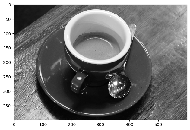
Consider the grayscale coffee image with resolution of 400 x 600 pixels, meaning it contains 240,000 pixels in total. Each pixel represents a grayscale value between 0 and 255, requiring 8 bits of storage per pixel. Consequently, the full image occupies approximately 240 KB of storage.
VQ Compression Steps#
The following steps demonstrate how VQ compression is performed on this image:
Block Partitioning: The image is divided into 2x2 blocks of pixels. This means each block contains 4 pixel values, and the total number of blocks is 200 x 300.
K-means Clustering: We apply the K-means clustering algorithm to the pixel blocks, treating each block as a vector in \(\mathbb{R}^4\) (four-dimensional space).
Choosing K = 4: This results in a significant reduction in quality, but a more significant reduction in storage.
Encoding Step: Each block of pixels is approximated by its closest cluster centroid, known as a codeword. The identity of the closest codeword for each block needs to be stored. This requires \(log_2(K)\) bits per block.
Decoding Step: To reconstruct the approximated image, the centroids are used to create the final image. This step is called the decoding step.
Storage Obligation#
When K is reduced to 4, the storage requirement the storage for the compressed image amounts to \(log_2(K)/(4 \times 8) = 1/16 = 0.0625\) of the original image, equating to 0.50 bits per pixel.
The crucial steps in VQ involve encoding each block to its nearest codeword and then decoding the image using these codewords, illustrating how K-means can facilitate significant compression in image storage.
import numpy as np
import matplotlib.pyplot as plt
from sklearn.cluster import KMeans
# from sklearn_extra.cluster import KMedoids
from skimage import io
from skimage import data
from skimage.color import rgb2gray
coffee = data.coffee()
img = rgb2gray(coffee)
m, n = img.shape
print(m,n,type(img[0,0]))
print(img.min(),img.max())
400 600 <class 'numpy.float64'>
0.0002827450980392157 1.0
io.imshow(img)
<matplotlib.image.AxesImage at 0x20a1f0aaf50>
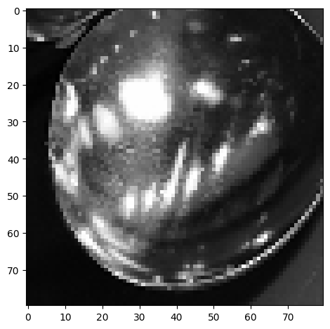
blk = img[250:330,320:400]
blk
io.imshow(blk)
<matplotlib.image.AxesImage at 0x20a200556f0>
Some utility functions
from skimage.util import view_as_windows as viewW
from skimage.util import view_as_blocks as viewB

def im2col_sliding_strided_v2(A, block_size, stepsize=1):
    a, b = block_size
    return viewW(A, (a,b)).reshape(-1,a*b).T[:,::stepsize]

def im2col_distinct(B, block_size):
    a, b = block_size
    return viewB(B, (a,b)).reshape(-1,a*b).T#[:,::stepsize]

def col2im_sliding(B, block_size, image_size):
    a, b = block_size
    m, n = image_size
    return B.reshape(n-b+1,m-a+1).T

def col2im_distinct(A, block_size, image_size):
    a, b = block_size
    m, n = image_size
    B = A.reshape((m//a,n//b,a,b)) #C = A.reshape((3,2,2,2))
    return B.transpose([0,2,1,3]).reshape(m,n)#B.reshape(nn-n+1,mm-m+1).T
A = np.arange(4*6).reshape(4,6)
patch_arr = viewB(A, (2,2))
print(A)
print(patch_arr.shape)
patch_arr
[[ 0  1  2  3  4  5]
 [ 6  7  8  9 10 11]
 [12 13 14 15 16 17]
 [18 19 20 21 22 23]]
(2, 3, 2, 2)
array([[[[ 0,  1],
         [ 6,  7]],

        [[ 2,  3],
         [ 8,  9]],

        [[ 4,  5],
         [10, 11]]],


       [[[12, 13],
         [18, 19]],

        [[14, 15],
         [20, 21]],

        [[16, 17],
         [22, 23]]]])
B = im2col_distinct(A,[2, 2])
print(A)
print(B)
[[ 0  1  2  3  4  5]
 [ 6  7  8  9 10 11]
 [12 13 14 15 16 17]
 [18 19 20 21 22 23]]
[[ 0  2  4 12 14 16]
 [ 1  3  5 13 15 17]
 [ 6  8 10 18 20 22]
 [ 7  9 11 19 21 23]]
C = col2im_distinct(B.T,[2, 2], [4, 6])
C
array([[ 0,  1,  2,  3,  4,  5],
       [ 6,  7,  8,  9, 10, 11],
       [12, 13, 14, 15, 16, 17],
       [18, 19, 20, 21, 22, 23]])
bs = [2, 2]
x = im2col_distinct(img,bs)
print(x.shape, x.shape[0]*x.shape[1], m*n/4)
(4, 60000) 240000 60000.0
k = 4
kmeans = KMeans(n_clusters=k, random_state=0).fit(x.T)
# clustering = KMedoids(n_clusters=k, random_state=0).fit(x.T)
Show code cell output
C:\Users\m.amintoosi\AppData\Roaming\Python\Python310\site-packages\sklearn\cluster\_kmeans.py:1412: FutureWarning: The default value of `n_init` will change from 10 to 'auto' in 1.4. Set the value of `n_init` explicitly to suppress the warning
  super()._check_params_vs_input(X, default_n_init=10)
print(kmeans.cluster_centers_.shape)
labels = kmeans.labels_
print(labels.shape)
cluster_centers = kmeans.cluster_centers_
cluster_centers
(4, 4)
(60000,)
array([[0.52268354, 0.52463973, 0.52423633, 0.52303693],
       [0.08968596, 0.08971989, 0.08917598, 0.08987512],
       [0.79994586, 0.80255419, 0.80365328, 0.80144409],
       [0.3172317 , 0.31510994, 0.31436142, 0.31667701]])
rec_img_centers = cluster_centers[labels]
print(rec_img_centers.shape)
(60000, 4)
rec_img_blk = col2im_distinct(rec_img_centers,bs,[m,n])
# print(y.shape,imc.shape,type(imc[0,0]))
io.imshow(rec_img_blk)
<matplotlib.image.AxesImage at 0x20a200e4820>
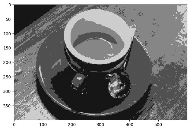
Image Compression Using kmeans#
X = img.reshape(-1,1)
kmeans = KMeans(n_clusters=4)
kmeans.fit(X)
labels = kmeans.labels_
cluster_centers = kmeans.cluster_centers_
# replacing each pixel with corresponding cluster center
rec_img_pixels = cluster_centers[labels]
rec_img_pixels = rec_img_pixels.reshape(img.shape)
plt.figure(figsize=(10, 5))
# plt.subplot(1, 3, 1)
# plt.axis("off")
# plt.imshow(img, cmap="gray")
plt.subplot(1, 2, 1)
plt.axis("off")
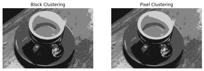
plt.imshow(rec_img_blk, cmap="gray", vmin=0, vmax=1)
plt.title('Block Clustering')
plt.subplot(1, 2, 2)
plt.axis("off")
plt.imshow(rec_img_pixels, cmap="gray", vmin=0, vmax=1)
plt.title('Pixel Clustering')
C:\Users\m.amintoosi\AppData\Roaming\Python\Python310\site-packages\sklearn\cluster\_kmeans.py:1412: FutureWarning: The default value of `n_init` will change from 10 to 'auto' in 1.4. Set the value of `n_init` explicitly to suppress the warning
  super()._check_params_vs_input(X, default_n_init=10)
Text(0.5, 1.0, 'Pixel Clustering')
cluster_centers
array([[0.52732396],
       [0.0897978 ],
       [0.80943031],
       [0.31605731]])