Dimensionality Reduction - Part 1#
Mahmood Amintoosi, Fall 2024
Computer Science Dept, Ferdowsi University of Mashhad
Principal Component Analysis#
In Depth: Principal Component Analysis, Python Data Science Handbook
-
Matrix Differentiation by Randal J. Barnes
Further Readning
An Introduction to Principal Component Analysis (PCA) with 2018 World Soccer Players Data, PDF
Using PCA to See Which Countries have Better Players for World Cup Games, PDF
Paper: Eigenbackground Revisited
Chapter 7 of Zaki
import numpy as np
import matplotlib.pyplot as plt
import seaborn as sb
import pandas as pd
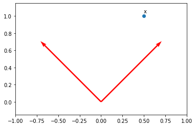
u0 = np.array([[1], [1]])
u0 = u0 / np.linalg.norm(u0)
# u0, np.linalg.norm(u0)
u1 = u0.copy()
u1[0] *= -1
u0, u1
(array([[0.70710678],
        [0.70710678]]),
 array([[-0.70710678],
        [ 0.70710678]]))
origin = np.array([0, 0])
plt.quiver(
    origin[0],
    origin[1],
    u0[0],
    u0[1],
    scale=1,
    scale_units="xy",
    angles="xy",
    color="r",
)
plt.quiver(
    origin[0],
    origin[1],
    u1[0],
    u1[1],
    scale=1,
    scale_units="xy",
    angles="xy",
    color="r",
)

x = np.array([0.5, 1])
x = np.reshape(x, (2, 1))
plt.scatter(x[0], x[1])
plt.axis("equal")
plt.axis([-1, 1, 0, 1])
plt.text(x[0], x[1]+0.04, "x")
Text([0.5], [1.04], 'x')
U = np.concatenate((u0, u1), axis=1)
U, x
(array([[ 0.70710678, -0.70710678],
        [ 0.70710678,  0.70710678]]),
 array([[0.5],
        [1. ]]))
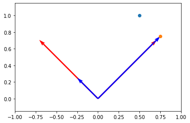
# eq 7.3, page 185 Zaki
a = U.T @ x
x, a, U @ a
(array([[0.5],
        [1. ]]),
 array([[1.06066017],
        [0.35355339]]),
 array([[0.5],
        [1. ]]))
origin = np.array([0, 0])
plt.quiver(
    origin[0],
    origin[1],
    u0[0],
    u0[1],
    scale=1,
    scale_units="xy",
    angles="xy",
    color="r",
)
plt.quiver(
    origin[0],
    origin[1],
    u1[0],
    u1[1],
    scale=1,
    scale_units="xy",
    angles="xy",
    color="r",
)
a0u0 = a[0] * u0
a1u1 = a[1] * u1
plt.quiver(
    origin[0],
    origin[1],
    a0u0[0],
    a0u0[1],
    scale=1,
    scale_units="xy",
    angles="xy",
    color="b",
)
plt.quiver(
    origin[0],
    origin[1],
    a1u1[0],
    a1u1[1],
    scale=1,
    scale_units="xy",
    angles="xy",
    color="b",
)

plt.scatter(x[0], x[1])
plt.axis("equal")
plt.axis([-1, 1, 0, 1])
(-1.0, 1.0, 0.0, 1.0)

U, x, a
(array([[ 0.70710678, -0.70710678],
        [ 0.70710678,  0.70710678]]),
 array([[0.5],
        [1. ]]),
 array([[1.06066017],
        [0.35355339]]))
u0 * a[0] + u1 * a[1], U @ a
(array([[0.5],
        [1. ]]),
 array([[0.5],
        [1. ]]))
# Eq 7.5
r = 1
Ur = U[:,0:r]
ar = a[:r]
x_prime = Ur@ar
x_prime
array([[0.75],
       [0.75]])
a[0]*u0, U[:,0:1]@a[:1], u0 @ a[:1], u0 @ a[0]
(array([[0.75],
        [0.75]]),
 array([[0.75],
        [0.75]]),
 array([[0.75],
        [0.75]]),
 array([0.75, 0.75]))
# x_prime is the projection of x onto the first r basis vectors
x_projected = Ur@ar
x_projected
array([[0.75],
       [0.75]])
origin = np.array([0, 0])
plt.quiver(
    origin[0],
    origin[1],
    u0[0],
    u0[1],
    scale=1,
    scale_units="xy",
    angles="xy",
    color="r",
)
plt.quiver(
    origin[0],
    origin[1],
    u1[0],
    u1[1],
    scale=1,
    scale_units="xy",
    angles="xy",
    color="r",
)
a0u0 = a[0] * u0
a1u1 = a[1] * u1
plt.quiver(
    origin[0],
    origin[1],
    a0u0[0],
    a0u0[1],
    scale=1,
    scale_units="xy",
    angles="xy",
    color="b",
)
plt.quiver(
    origin[0],
    origin[1],
    a1u1[0],
    a1u1[1],
    scale=1,
    scale_units="xy",
    angles="xy",
    color="b",
)

plt.scatter(x[0], x[1])
plt.scatter(x_projected[0], x_projected[1])
plt.axis("equal")
plt.axis([-1, 1, 0, 1])
(-1.0, 1.0, 0.0, 1.0)
Page 189 of Zaki
We also assume that the data matrix D has been centered by subtracting the mean \(\mu\)
\(X \equiv D\)
\( mean\_X \equiv \mu\)
\( Z \equiv X\_centered \equiv \bar{D}\)
Algorithm 7.1, page 199 of Zaki book, Slide 16 of Chap 7
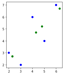
X = np.array([[2, 3], [3, 2], [4, 6], [5, 4], [6, 7]])

# Step 1
mean_X = np.mean(X, axis=0)

# Step 2
Z = X - mean_X
print(Z.shape)

# Step 3
Sigma = 1 / X.shape[0] * Z.T @ Z
Sigma
(5, 2)
array([[2.  , 2.  ],
       [2.  , 3.44]])
\( \Sigma \approx Cov\)
# covariance, function needs samples as columns

# cov_mat = np.cov(Z.T)
# cov_mat
# Sigma = np.zeros((2,2))
# for i in range(X.shape[0]):
#     xi = Z[i]
#     Sigma += xi.reshape(2,1)*xi
# Sigma /= (X.shape[0])
# Sigma
# Step 4, 5
lambdas, U = np.linalg.eigh(Sigma)
lambdas, U
(array([0.59434716, 4.84565284]),
 array([[-0.81814408,  0.57501327],
        [ 0.57501327,  0.81814408]]))
# eigen_values, eigen_vectors = np.linalg.eigh(Sigma)
# eigen_values, eigen_vectors
lambda0 = lambdas[0]
u0 = U[:, 0:1]
print(u0)
print(Sigma @ u0)
print(lambda0 * u0)
[[-0.81814408]
 [ 0.57501327]]
[[-0.48626161]
 [ 0.34175751]]
[[-0.48626161]
 [ 0.34175751]]
U @ np.diag(lambdas) @ np.linalg.inv(U)
array([[2.  , 2.  ],
       [2.  , 3.44]])
# Steps 4, continue ... (Sorting)
sorted_index = np.argsort(lambdas)[::-1]
lambdas = lambdas[sorted_index]
U = U[:, sorted_index]
lambdas, U
(array([4.84565284, 0.59434716]),
 array([[ 0.57501327, -0.81814408],
        [ 0.81814408,  0.57501327]]))
Steps 6 & 7 is omitted
num_components = 1
# Step 8
Ur = U[:, 0:num_components]
Ur
array([[0.57501327],
       [0.81814408]])
Step 9: X_projected = A
There is mistake in the Algorithm in slides, x should be replaced with \(\bar{x}\)
X_projected = Z @ Ur
X_projected
array([[-2.40416306],
       [-2.40416306],
       [ 1.13137085],
       [ 0.42426407],
       [ 3.25269119]])
X_reconstructed = X_projected @ Ur.T + mean_X
X_reconstructed
array([[2.3, 2.7],
[2.3, 2.7],
[4.8, 5.2],
[4.3, 4.7],
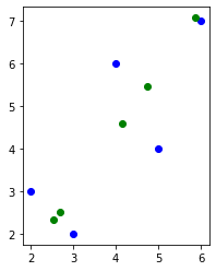
[6.3, 6.7]])
fig = plt.figure()
plt.scatter(X[:, 0], X[:, 1], c="blue")
plt.scatter(X_reconstructed[:, 0], X_reconstructed[:, 1], c="green")
ax = plt.gca()
ax.set_aspect("equal", adjustable="box")
plt.draw()
def PCA(X, num_components):
    # num_components = r
    # Step-1
    mean_X = np.mean(X, axis=0)
    Z = X - mean_X

    # Step-2
    # covariance, function needs samples as columns
    cov_mat = np.cov(Z.T)

    # Step-3
    lambdas, U = np.linalg.eigh(cov_mat)

    # Step-4
    sorted_index = np.argsort(lambdas)[::-1]
    # sorted_eigenvalues = eigen_values[sorted_index]
    U = U[:, sorted_index]

    # Step-8
    Ur = U[:, 0:num_components]

    # Step-9, A
    X_projected = Z @ Ur

    X_reconstructed = X_projected @ Ur.T + mean_X

    return X_projected, X_reconstructed
# Applying it to PCA function
X_projected, X_reconstructed = PCA(X, 1)

fig = plt.figure()
plt.scatter(X[:, 0], X[:, 1], c="blue")
plt.scatter(X_reconstructed[:, 0], X_reconstructed[:, 1], c="green")
ax = plt.gca()
ax.set_aspect("equal", adjustable="box")
plt.draw()
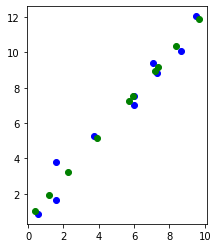
w0, w1 = 2, 1
N = 10

# Data Generation
np.random.seed(42)
x = np.random.rand(N, 1)*10

epsilon = np.random.randn(N, 1)
y = w0 + w1 * x + epsilon
X = np.hstack([x, y])
X.shape
(10, 2)
X_projected, X_reconstructed = PCA(X, 1)

fig = plt.figure()
plt.scatter(X[:, 0], X[:, 1], c="blue")
plt.scatter(X_reconstructed[:, 0], X_reconstructed[:, 1], c="green")
ax = plt.gca()
ax.set_aspect("equal", adjustable="box")
plt.draw()