Introduction to Pytorch & Neural Networks

Mahmood Amintoosi, Spring 2024

Computer Science Dept, Ferdowsi University of Mashhad

I should mention that the original material was from Tomas Beuzen’s course.

Lecture Outline

---

• Lecture Learning Objectives
• Imports
• 1. Introduction
• 2. PyTorch's Tensor
• 3. Neural Network Basics
• 4. Activation Functions
• 5. Neural Network Classification
• 6. Lecture Exercise: True/False Questions
• 7. The Lecture in Three Conjectures

Lecture Learning Objectives

---

• Describe the difference between numpy and torch arrays (np.array vs. torch.Tensor)

• Explain fundamental concepts of neural networks such as layers, nodes, activation functions, etc.

• Create a simple neural network in PyTorch for regression or classification

Imports

---

# Auto-setup when running on Google Colab
import os
if 'google.colab' in str(get_ipython()) and not os.path.exists('/content/neural-networks'):
    !git clone -q https://github.com/fum-cs/neural-networks.git /content/neural-networks
    !pip --quiet install -r /content/neural-networks/requirements_colab.txt
    %cd neural-networks/notebooks

import warnings
warnings.filterwarnings('ignore')
import sys
import numpy as np
import pandas as pd
import torch
from torchsummary import summary
from torch import nn, optim
from torch.utils.data import DataLoader, TensorDataset
from sklearn.datasets import make_regression, make_circles, make_blobs
from sklearn.preprocessing import StandardScaler
from sklearn.linear_model import LinearRegression
from utils.plotting import *
import plotly.io as pio
pio.renderers.default = 'notebook'

1. Introduction

---

• PyTorch is a Python-based tool for scientific computing that provides several main features:

  • torch.Tensor, an n-dimensional array similar to that of numpy, but which can run on GPUs

  • Computational graphs for building neural networks

  • Automatic differentiation for training neural networks (more on this next lecture)

• You can install PyTorch from: https://pytorch.org/

2. PyTorch’s Tensor

---

• In PyTorch a tensor is just like NumPy’s ndarray that we have become so familiar with.

• A key difference between PyTorch’s torch.Tensor and numpy’s np.array is that torch.Tensor was constructed to integrate with GPUs and PyTorch’s computational graphs (more on that next lecture though)

2.1. ndarray vs tensor

• Creating and working with tensors is much the same as with numpy ndarrays

• You can create a tensor with torch.tensor():

tensor_1 = torch.tensor([1, 2, 3])
tensor_2 = torch.tensor([1, 2, 3], dtype=torch.float32)
tensor_3 = torch.tensor(np.array([1, 2, 3]))

for t in [tensor_1, tensor_2, tensor_3]:
    print(f"{t}, dtype: {t.dtype}")

tensor([1, 2, 3]), dtype: torch.int64
tensor([1., 2., 3.]), dtype: torch.float32
tensor([1, 2, 3], dtype=torch.int32), dtype: torch.int32

• PyTorch also comes with most of the numpy functions we’re already familiar with:

torch.zeros(2, 2)  # zeroes

tensor([[0., 0.],
        [0., 0.]])

torch.ones(2, 2)  # ones

tensor([[1., 1.],
        [1., 1.]])

torch.randn(3, 2)  # random normal

tensor([[ 0.3388,  0.0180],
        [-0.1241,  0.9065],
        [-1.6244,  0.1037]])

torch.rand(2, 3, 2)  # rand uniform

tensor([[[0.8185, 0.1055],
         [0.7195, 0.2424],
         [0.8114, 0.7107]],

        [[0.8324, 0.9311],
         [0.1115, 0.8091],
         [0.0066, 0.2076]]])

• Just like in NumPy we can look at the shape of a tensor with the .shape attribute:

x = torch.rand(2, 3, 2, 2)
x.shape

torch.Size([2, 3, 2, 2])

x.ndim

4

2.2. Tensors and Data Types

• Different dtypes have different memory and computational implications (see the end of Lecture 1 for more)

• In Pytorch we’ll be building networks that require thousands or even millions of floating point calculations!

• In such cases, using a smaller dtype like float32 can significantly speed up computations and reduce memory requirements

• The default float dtype in pytorch float32, as opposed to numpy’s float64

• In fact some operations in Pytorch will even throw an error if you pass a high-memory dtype!

print(np.array([3.14159]).dtype)
print(torch.tensor([3.14159]).dtype)

float64
torch.float32

• But just like in numpy, you can always specify the particular dtype you want using the dtype argument:

print(torch.tensor([3.14159], dtype=torch.float64).dtype)

torch.float64

2.3. Operations on Tensors

• Tensors operate just like ndarrays and have a variety of familiar methods that can be called off them:

a = torch.rand(1, 3)
b = torch.rand(3, 1)

a + b  # broadcasting betweean a 1 x 3 and 3 x 1 tensor

tensor([[0.6376, 0.8497, 0.5364],
        [0.1417, 0.3538, 0.0404],
        [0.8795, 1.0915, 0.7782]])

a * b

tensor([[5.5718e-02, 1.6878e-01, 1.7360e-03],
        [3.8856e-03, 1.1771e-02, 1.2106e-04],
        [8.0994e-02, 2.4535e-01, 2.5235e-03]])

a.mean()

tensor(0.1415)

a.sum()

tensor(0.4244)

2.4. Indexing

• Once again, same as NumPy!

X = torch.rand(5, 2)
print(X)

tensor([[0.5512, 0.5119],
        [0.8011, 0.4224],
        [0.1395, 0.0438],
        [0.5987, 0.7250],
        [0.2124, 0.4778]])

print(X[0, :])
print(X[0])
print(X[:, 0])

tensor([0.5512, 0.5119])
tensor([0.5512, 0.5119])
tensor([0.5512, 0.8011, 0.1395, 0.5987, 0.2124])

2.5. Numpy Bridge

• Sometimes we might want to convert a tensor back to a NumPy array

• We can do that using the .numpy() method

X = torch.rand(3,3)
print(type(X))
X_numpy = X.numpy()
print(type(X_numpy))

<class 'torch.Tensor'>
<class 'numpy.ndarray'>

2.6. GPU and CUDA Tensors

• GPU is a graphical processing unit (as opposed to a CPU: central processing unit)

• GPUs were originally developed for gaming, they are very fast at performing operations on large amounts of data by performing them in parallel (think about updating the value of all pixels on a screen very quickly as a player moves around in a game)

• More recently, GPUs have been adapted for more general purpose programming

• Neural networks can typically be broken into smaller computations that can be performed in parallel on a GPU

• PyTorch is tightly integrated with CUDA - a software layer that facilitates interactions with a GPU (if you have one)

• You can check if you have GPU capability using:

torch.cuda.is_available()  # my MacBook Pro does not have a GPU

False

• When training on a machine that has a GPU, you need to tell PyTorch you want to use it

• You’ll see the following at the top of most PyTorch code:

device = torch.device('cuda' if torch.cuda.is_available() else 'cpu')
print(device)

cpu

• You can then use the device argument when creating tensors to specify whether you wish to use a CPU or GPU

• Or if you want to move a tensor between the CPU and GPU, you can use the .to() method:

X = torch.rand(2, 2, 2, device=device)
print(X.device)

cpu

# X.to('cuda')  # this would give an error for me so I'm commenting out

• We’ll revisit GPUs later in the course when we are working with bigger datasets and more complex networks

• For now, we can work on the CPU just fine

3. Neural Network Basics

---

• You’ve already learned about several machine learning algorithms (kNN, Random Forest, SVM, etc.)

• Neural networks are simply another algorithm and actually one of the simplest in my opinion!

• As we’ll see, a neural network is just a sequence of linear and non-linear transformations

• Often you see something like this when learning about/using neural networks:

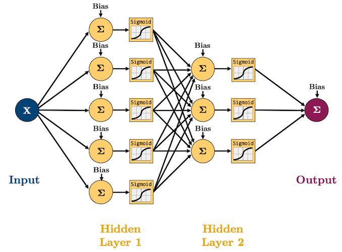
• So what on Earth does that all mean? Well we are going to build up some intuition one step at a time

3.1. Simple Linear Regression with a Neural Network

• Let’s create a simple regression dataset with 500 observations:

X, y = make_regression(n_samples=500, n_features=1, random_state=0, noise=10.0)
plot_regression(X, y)

• We know how to fit a simple linear regression to this data using sklearn:

sk_model = LinearRegression().fit(X, y)
plot_regression(X, y, sk_model.predict(X))

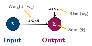
• Here are the parameters of that fitted line:

print(f"w_0: {sk_model.intercept_:.2f} (bias/intercept)")
print(f"w_1: {sk_model.coef_[0]:.2f}")

w_0: -0.77 (bias/intercept)
w_1: 45.50

• As an equation, that looks like this:

\[\hat{y}=-0.77 + 45.50X\]

• Or in matrix form:

\[\begin{split}\begin{bmatrix} \hat{y_1} \\ \hat{y_2} \\ \vdots \\ \hat{y_n} \end{bmatrix}=\begin{bmatrix} 1 & x_1 \\ 1 & x_2 \\ \vdots & \vdots \\ 1 & x_n \end{bmatrix} \begin{bmatrix} -0.77 \\ 45.55 \end{bmatrix}\end{split}\]

• Or in graph form I’ll represent it like this:

3.2. Linear Regression with a Neural Network in PyTorch

• So let’s implement the above in PyTorch to start gaining an intuition about neural networks!

• Every neural network model you build in PyTorch will inherit from torch.nn.Module

• Inheritance allows us to inherit commonly needed functionality without having to write code ourselves! W3 Schools has a good mini tutorial for class inhertance in Python.

We’ll explore torch.nn.Module more in the lab but if it helps, think about sklearn models: they all inherit common methods like .fit(), .predict(), .score(), etc. When creating a neural network, we define our own architecture but still want common functionality which we inherit from torch.nn.Module.

• Let’s create a model called linearRegression and then I’ll talk you through the syntax:

class linearRegression(nn.Module):  # our class inherits from nn.Module and we can call it anything we like
    def __init__(self, input_size, output_size):
        super().__init__()                                # super().__init__() makes our class inherit everything from torch.nn.Module
        self.linear = nn.Linear(input_size, output_size)  # this is a simple linear layer: wX + b

    def forward(self, x):
        out = self.linear(x)
        return out

Let’s step through the above:

class linearRegression(nn.Module):
    def __init__(self, input_size, output_size):
        super().__init__() 

Here we’re creating a class called linearRegression and inheriting the methods and attributes of nn.Module (hint: try typing help(linearRegression) to see all the things we inheritied from nn.Module).

        self.linear = nn.Linear(input_size, output_size)

Here we’re defining a “Linear” layer, which just means wX + b, i.e., the weights of the network, multiplied by the input features plus the bias.

    def forward(self, x):
        out = self.linear(x)
        return out

PyTorch networks created with nn.Module must have a forward() method. It accepts the input data x and passes it through the defined operations. In this case, we are passing x into our linear layer and getting an output out.

• After defining the model class, we can create an instance of that class:

model = linearRegression(input_size=1, output_size=1)

• We can check out our model using print():

print(model)

linearRegression(
  (linear): Linear(in_features=1, out_features=1, bias=True)
)

• Or the more useful summary() (which we imported at the top of this notebook with from torchsummary import summary):

summary(model, (1,));

----------------------------------------------------------------
        Layer (type)               Output Shape         Param #
================================================================
            Linear-1                    [-1, 1]               2
================================================================
Total params: 2
Trainable params: 2
Non-trainable params: 0
----------------------------------------------------------------
Input size (MB): 0.00
Forward/backward pass size (MB): 0.00
Params size (MB): 0.00
Estimated Total Size (MB): 0.00
----------------------------------------------------------------

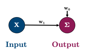
• Notice how we have two parameters? We have one for the weight (w1) and one for the bias (w0)

• These were initialized randomly by PyTorch when we created our model. They can be accessed with model.state_dict():

model.state_dict()

OrderedDict([('linear.weight', tensor([[0.3072]])),
             ('linear.bias', tensor([-0.9891]))])

• Okay, before we move on, our x and y data are currently numpy arrays but they need to be PyTorch tensors

• Let’s convert them:

X_t = torch.tensor(X, dtype=torch.float32)  # I'll explain requires_grad next lecture
y_t = torch.tensor(y, dtype=torch.float32)

• We have a working model right now and could tell it to give us some output with this syntax:

y_p = model(X_t[0]).item()
print(f"Predicted: {y_p:.2f}")
print(f"   Actual: {y[0]:.2f}")

Predicted: -0.80
   Actual: 31.08

• Our prediction is pretty bad because our model is not trained/fitted yet!

• As we learned in the past few lectures, to fit our model we need:

  1. a loss function (called “criterion” in PyTorch) to tell us how good/bad our predictions are - we’ll use mean squared error, torch.nn.MSELoss()

  2. an optimization algorithm to help optimise model parameters - we’ll use GD, torch.optim.SGD()

LEARNING_RATE = 0.1
criterion = nn.MSELoss()  # loss function
optimizer = torch.optim.SGD(model.parameters(), lr=LEARNING_RATE)  # optimization algorithm is SGD

• Before we train I’m going to create a “data loader” to help batch my data

• Data loaders are just generators that yield data to us on request.

• We’ll use a BATCH_SIZE = 50 (which should give us 10 batches because we have 500 data points)

BATCH_SIZE = 50
dataset = TensorDataset(X_t, y_t)
dataloader = DataLoader(dataset, batch_size=BATCH_SIZE, shuffle=True)

• We should have 10 batches:

print(f"Total number of batches: {len(dataloader)}")

Total number of batches: 10

• We can look at a batch using this syntax:

XX, yy = next(iter(dataloader))
print(f" Shape of feature data (X) in batch: {XX.shape}")
print(f"Shape of response data (y) in batch: {yy.shape}")

 Shape of feature data (X) in batch: torch.Size([50, 1])
Shape of response data (y) in batch: torch.Size([50])

• With those, let’s train our simple network for 5 epochs of SGD!

I’ll explain all the code here next lecture but scan throught it, it’s not too hard to see what’s going on!

def trainer(model, criterion, optimizer, dataloader, epochs=5, verbose=True):
    """Simple training wrapper for PyTorch network."""
    
    for epoch in range(epochs):
        losses = 0
        for X, y in dataloader:
            optimizer.zero_grad()       # Clear gradients w.r.t. parameters
            y_hat = model(X).flatten()  # Forward pass to get output
            loss = criterion(y_hat, y)  # Calculate loss
            loss.backward()             # Getting gradients w.r.t. parameters
            optimizer.step()            # Update parameters
            losses += loss.item()       # Add loss for this batch to running total
        if verbose: print(f"epoch: {epoch + 1}, loss: {losses / len(dataloader):.4f}")
   
trainer(model, criterion, optimizer, dataloader, epochs=5, verbose=True)

epoch: 1, loss: 648.7896
epoch: 2, loss: 99.0878
epoch: 3, loss: 94.1367
epoch: 4, loss: 93.6165
epoch: 5, loss: 93.4385

• Now our model has been trained, our parameters should be different than before:

model.state_dict()

OrderedDict([('linear.weight', tensor([[45.7395]])),
             ('linear.bias', tensor([-0.7178]))])

• Comparing to our sklearn model, we get the same answer:

pd.DataFrame({"w0": [sk_model.intercept_, model.state_dict()['linear.bias'].item()],
              "w1": [sk_model.coef_[0], model.state_dict()['linear.weight'].item()]},
             index=['sklearn', 'pytorch']).round(2)

	w0	w1
sklearn	-0.77	45.50
pytorch	-0.72	45.74

• We got pretty close! We could do better by changing the number of epochs or the learning rate

• So here is our simple network once again:

• By the way, check out what happens if we run trainer() again:

trainer(model, criterion, optimizer, dataloader, epochs=5, verbose=True)

epoch: 1, loss: 93.5241
epoch: 2, loss: 94.1431
epoch: 3, loss: 93.9253
epoch: 4, loss: 93.4623
epoch: 5, loss: 93.8662

• Our model continues where we left off!

• This may or may not be what you want. We can start from scratch by re-making our model and optimizer.

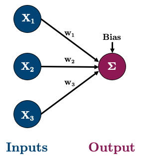
3.3. Multiple Linear Regression with a Neural Network

• Okay, let’s do a multiple linear regression now with 3 features

• So our network will look like this:

• Let’s go ahead and create some data:

# Create dataset
X, y = make_regression(n_samples=500, n_features=3, random_state=0, noise=10.0)
X_t = torch.tensor(X, dtype=torch.float32)
y_t = torch.tensor(y, dtype=torch.float32)
# Create dataloader
dataset = TensorDataset(X_t, y_t)
dataloader = DataLoader(dataset, batch_size=BATCH_SIZE, shuffle=True)

• And let’s create the above model:

model = linearRegression(input_size=3, output_size=1)

• We should now have 4 parameters (3 weights and 1 bias)

summary(model, (3,));

----------------------------------------------------------------
        Layer (type)               Output Shape         Param #
================================================================
            Linear-1                    [-1, 1]               4
================================================================
Total params: 4
Trainable params: 4
Non-trainable params: 0
----------------------------------------------------------------
Input size (MB): 0.00
Forward/backward pass size (MB): 0.00
Params size (MB): 0.00
Estimated Total Size (MB): 0.00
----------------------------------------------------------------

• Looks good to me! Let’s train the model and then compare it to sklearn’s LinearRegression():

criterion = nn.MSELoss()
optimizer = torch.optim.SGD(model.parameters(), lr=LEARNING_RATE)
trainer(model, criterion, optimizer, dataloader, epochs=5, verbose=True)

epoch: 1, loss: 1007.8107
epoch: 2, loss: 110.3681
epoch: 3, loss: 102.1059
epoch: 4, loss: 101.9216
epoch: 5, loss: 102.1261

sk_model = LinearRegression().fit(X, y)
pd.DataFrame({"w0": [sk_model.intercept_, model.state_dict()['linear.bias'].item()],
              "w1": [sk_model.coef_[0], model.state_dict()['linear.weight'][0, 0].item()],
              "w2": [sk_model.coef_[1], model.state_dict()['linear.weight'][0, 1].item()],
              "w3": [sk_model.coef_[2], model.state_dict()['linear.weight'][0, 2].item()]},
             index=['sklearn', 'pytorch']).round(2)

	w0	w1	w2	w3
sklearn	0.43	0.62	55.99	11.14
pytorch	0.82	0.60	56.06	11.19

3.4. Non-linear Regression with a Neural Network

• Okay so we can make a simple network to imitate simple and multiple linear regression

• You’re probably thinking, so what? But we’re getting to the good stuff I promise!

• For example, what happens when we have more complicated datasets like this?

# Create dataset
np.random.seed(2020)
X = np.sort(np.random.randn(500))
y = X ** 2 + 15 * np.sin(X) **3
X_t = torch.tensor(X[:, None], dtype=torch.float32)
y_t = torch.tensor(y, dtype=torch.float32)
# Create dataloader
dataset = TensorDataset(X_t, y_t)
dataloader = DataLoader(dataset, batch_size=BATCH_SIZE, shuffle=True)
plot_regression(X, y, y_range=[-25, 25], dy=5)

• This is obviously non-linear, and we need to introduce some non-linearities into our network

• These non-linearities are what make neural networks so powerful and they are called “activation functions”

• We are going to create a new model class that includes a non-linearity - a sigmoid function:

\[S(X)=\frac{1}{1+e^{-x}}\]

def sigmoid(x):
    return 1 / (1 + np.exp(-x))

xs = np.linspace(-15, 15, 100)
plot_regression(xs, [0], sigmoid(xs), x_range=[-5, 5], y_range=[0, 1], dy=0.2)

• We’ll talk more about activation functions later, but note how the sigmoid function non-linearly maps x to a value between 0 and 1

• Okay, so let’s create the following network:

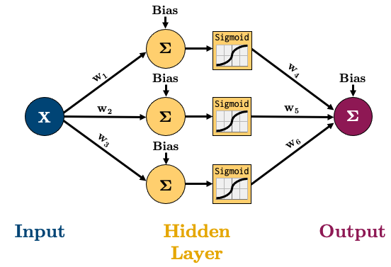
• All this means is that the value of each node in the hidden layer will be transformed by the “activation function”, thus introducing non-linear elements to our model!

• There’s two main ways of creating the above model in PyTorch, I’ll show you both:

class nonlinRegression(nn.Module):
    def __init__(self, input_size, hidden_size, output_size):
        super().__init__()
        self.hidden = nn.Linear(input_size, hidden_size)
        self.output = nn.Linear(hidden_size, output_size)
        self.sigmoid = nn.Sigmoid()

    def forward(self, x):
        x = self.hidden(x)       # input -> hidden layer
        x = self.sigmoid(x)      # sigmoid activation function in hidden layer
        x = self.output(x)       # hidden -> output layer
        return x

• Note how our forward() method now passes x through the nn.Sigmoid() function after the hidden layer

• The above method is very clear and flexible, but I prefer using nn.Sequential() to combine my layers together in the constructor:

class nonlinRegression(nn.Module):
    def __init__(self, input_size, hidden_size, output_size):
        super().__init__()
        self.main = torch.nn.Sequential(
            nn.Linear(input_size, hidden_size),  # input -> hidden layer
            nn.Sigmoid(),                        # sigmoid activation function in hidden layer
            nn.Linear(hidden_size, output_size)  # hidden -> output layer
        )

    def forward(self, x):
        x = self.main(x)
        return x

• Let’s make an instance of our new class and confirm it has 10 parameters (6 weights + 4 biases):

model = nonlinRegression(1, 3, 1)
summary(model, (1,))

----------------------------------------------------------------
        Layer (type)               Output Shape         Param #
================================================================
            Linear-1                    [-1, 3]               6
           Sigmoid-2                    [-1, 3]               0
            Linear-3                    [-1, 1]               4
================================================================
Total params: 10
Trainable params: 10
Non-trainable params: 0
----------------------------------------------------------------
Input size (MB): 0.00
Forward/backward pass size (MB): 0.00
Params size (MB): 0.00
Estimated Total Size (MB): 0.00
----------------------------------------------------------------

• Okay, let’s train:

criterion = nn.MSELoss()
optimizer = torch.optim.SGD(model.parameters(), lr=0.3)
trainer(model, criterion, optimizer, dataloader, epochs=10, verbose=True)

epoch: 1, loss: 32.5818
epoch: 2, loss: 14.8140
epoch: 3, loss: 7.6448
epoch: 4, loss: 5.2685
epoch: 5, loss: 4.8211
epoch: 6, loss: 4.7319
epoch: 7, loss: 4.4413
epoch: 8, loss: 4.2567
epoch: 9, loss: 4.3213
epoch: 10, loss: 4.2639

y_p = model(X_t).detach().numpy().squeeze()
plot_regression(X, y, y_p, y_range=[-25, 25], dy=5)

• Take a look at those non-linear predictions! Cool!

• Our model is not great and we could make it better soon by adjusting the learning rate, the number of nodes, and the number of epochs

• But I really want you to see how each of our hidden nodes is “engineering a non-linear feature” to be used for the predictions, check it out:

plot_nodes(X, y_p, model)

3.5. Multi Layer Perceptron

• You’ve probably heard the magic term “MLP” and you’re about to find out what it means!

• Really, it’s just a neural network with more than 1 hidden layer! Easy!

• Let’s create an “MLP” network of 2 layers:

class multiLayerRegression(nn.Module):
    def __init__(self, input_size, hidden_size_1, hidden_size_2, output_size):
        super().__init__()
        self.main = nn.Sequential(
            nn.Linear(input_size, hidden_size_1),
            nn.Sigmoid(),
            nn.Linear(hidden_size_1, hidden_size_2),
            nn.Sigmoid(),
            nn.Linear(hidden_size_2, output_size)
        )

    def forward(self, x):
        out = self.main(x)
        return out

model = multiLayerRegression(1, 5, 3, 1)
optimizer = torch.optim.SGD(model.parameters(), lr=0.3)
trainer(model, criterion, optimizer, dataloader, epochs=20, verbose=False)
plot_regression(X, y, model(X_t).detach(), y_range=[-25, 25], dy=5)

• But just because the network has more layer, doesn’t always mean it’s better!

4. Activation Functions

---

• As we learned above, activation functions are what allow us to model complex, non-linear functions

• There are many different activations functions:

functions = [torch.nn.Sigmoid, torch.nn.Tanh, torch.nn.Softplus, torch.nn.ReLU, torch.nn.LeakyReLU, torch.nn.SELU]
plot_activations(torch.linspace(-6, 6, 100), functions)

• Activation functions should be non-linear and tend to be monotonic and continuously differentiable (smooth)

• But as you can see with the ReLU function above, that’s not always the case!

• I wanted to point this out because it highlights how much of an art deep learning really is.

• Here’s a great quote from Yoshua Bengio (famous for his work in AI and deep learning) on his group experimenting with ReLU:

“…one of the biggest mistakes I made was to think, like everyone else in the 90s, that you needed smooth non-linearities in order for backpropagation to work. because I thought that if we had something like rectifying nonlinearities, where you have a flat part, that it would be really hard to train, because the derivative would be zero in so many places. And when we started experimenting with ReLU, with deep nets around 2010, I was obsessed with the idea that, we should be careful about whether neurons won’t saturate too much on the zero part. But in the end, it turned out that, actually, the ReLU was working a lot better than the sigmoids and tanh, and that was a big surprise…it turned out to work better, whereas I thought it would be harder to train!”

• Anyway, TL;DR ReLU is probably the most popular these days, but you can treat activation functions as hyperparams (to be optimized)

5. Lecture Exercise: True/False Questions

---

Answer True/False for the following:

1. Neural networks can be used for both regression and classification. (True)

2. For fully connected neural networks, the number of parameters \(\geq\) the number of features. (True)

3. Neural networks are parametric models. (True)

4. Any neural network with 3 hidden layers will have more parameters than any neural network with 2 hidden layers. (False)

5. The architecture of a neural network (number of hidden layers and hidden nodes) is a hyperparameter. (True)

6. Like linear regression or logistic regression, with neural networks we can interpret each feature’s weight value as a measure of the feature’s importance. (False)

6. The Lecture in Three Conjectures

---

1. PyTorch is a neural network software based on “tensors” (like NumPy arrays on steroids).

2. Neural Networks are simply:

   • Composed of an input layer, 1 or more hidden layers, and an output layer, each with 1 or more nodes.

   • The number of nodes in the Input/Output layers is defined by the problem/data. Hidden layers can have an arbitrary number of nodes.

   • Activation functions in the hidden layers help us model non-linear data.

   • Feed-forward neural networks are just a combination of simple linear and non-linear operations.

3. Activation functions allow the network to learn non-linear function