
Appendix A: Gradients Review#
Introduction#
This short appendix provides a refresher on gradients and calculus. Here we’ll cover the basics of the subject in this appendix. This material has been modified after material originally created by Mike Gelbart.
Show code cell source
# Auto-setup when running on Google Colab
import os
if 'google.colab' in str(get_ipython()) and not os.path.exists('/content/neural-networks'):
    !git clone -q https://github.com/fum-cs/neural-networks.git /content/neural-networks
    !pip --quiet install -r /content/neural-networks/requirements_colab.txt
    %cd neural-networks/notebooks
Show code cell content
import numpy as np
from scipy.optimize import minimize
import matplotlib.pyplot as plt
from mpl_toolkits.mplot3d import Axes3D
from skimage import data
from skimage.color import rgb2gray
from skimage.filters import gaussian

plt.style.use('ggplot')
plt.rcParams.update({'font.size': 16,
                     'axes.labelweight': 'bold',
                     'axes.grid': False,
                     'figure.figsize': (8,6)})
import plotly.io as pio
pio.renderers.default = 'notebook'
Functions of Multiple Variables#
We can write such a function as \(f(x,y,z)\) (for 3 inputs) or \(f(x)\) if \(x\) is a vector.
Example: \(f(x,y,z) = x^2 + y^2 + e^z + x^z + xyz\).
def f(x, y, z):
    return x**2 + y**2 + np.exp(z) + np.power(x,z) + x*y*z

f(1,2,3)
32.08553692318767
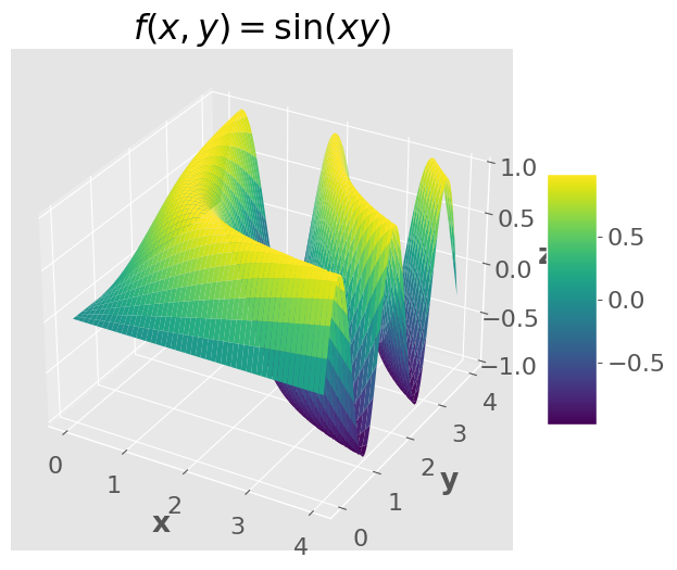
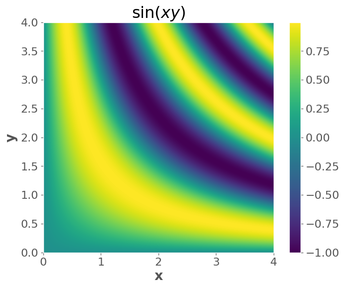
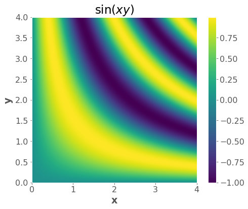
Another example: \(f(x,y) = \sin(xy)\)
We can visualize functions of two variables, but it gets much harder after that.
import numpy as np
import matplotlib.pyplot as plt

# Define the function
f = lambda x, y: np.sin(x * y)

# Create the grid
x = np.linspace(0, 4, 1000)
y = np.linspace(0, 4, 1000)
xx, yy = np.meshgrid(x, y)
zz = f(xx, yy)

# Create the 3D plot
fig = plt.figure()
ax = fig.add_subplot(111, projection='3d')

# Plot the surface with the 'plasma' colormap
surf = ax.plot_surface(xx, yy, zz, cmap='viridis')

# Set labels and title
ax.set_xlabel("x")
ax.set_ylabel("y")
ax.set_zlabel("z")
ax.set_title("$f(x,y) = \sin(xy)$")

# Add a colorbar for the 3D plot
fig.colorbar(surf, ax=ax, shrink=0.5, aspect=5)

plt.show()

# Create the 2D plot
plt.imshow(zz, extent=(np.min(x), np.max(x), np.min(y), np.max(y)), origin="lower")
plt.xlabel("x")
plt.ylabel("y")
plt.title("$\sin(xy)$")
plt.colorbar()
plt.show()
Vector-valued Functions#
You may not have encountered these yet in MDS.
These are functions with multiple outputs (and may or may not have multiple inputs).
Example with 1 input and 3 outputs:
Example with 3 inputs and 4 outputs:
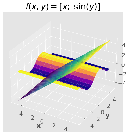
Example with 2 inputs and 2 outputs:
Show code cell content
def f(x, y):
    return np.array([x, np.sin(y)])


f(2, 10)
array([ 2. , -0.54402111])
We can visualize functions with two outputs (and two inputs), but it gets much harder after that.
Show code cell content
x = np.linspace(-5, 5, 20)
y = np.linspace(-5, 5, 20)
xx, yy = np.meshgrid(x, y)
zz = f(xx, yy)

# Create the 3D plot
fig = plt.figure()
ax = fig.add_subplot(111, projection='3d')

# Plot the surface
ax.plot_surface(xx, yy, zz[0], cmap='viridis')  # Plot x component
ax.plot_surface(xx, yy, zz[1], cmap='plasma')  # Plot sin(y) component

# Set labels and title
ax.set_xlabel("x")
ax.set_ylabel("y")
ax.set_zlabel("z")
ax.set_title("$f(x,y) = [x; \; \sin(y)]$")

plt.show()
Show code cell content
plt.quiver(xx, yy, zz[0], zz[1])
# plt.axis('square');
plt.xlabel("x")
plt.ylabel("y")
plt.title("$f(x,y) = [x; \; \sin(y)]$")
plt.show()
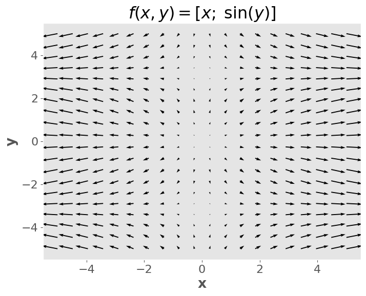
Notes:
For a fixed \(y\), when \(x\) grows, the \(x\)-component of the output grows (horizontal length of the arrows)
A similar argument can be made for \(y\).
It’s not always the case that the number of inputs equals the number of outputs - this is a special case!
But it’s a very important special case, as we’ll see below.
What it means is that the “input space” and the “output space” are the same.
Which allows for this kind of visualization.
(optional) It’s not always the case that the \(i\)th component of the output depends on the \(i\)th component of the inputs - this is also a special case!
Partial Derivatives#
A partial derivative is just a derivative of a multivariable function with respect to one of the input variables.
When taking this derivative, we treat all the other variables as constants.
Example: let \(f(x,y,z) = x^2 + y^2 + e^x + x^z + xyz\), let’s compute \(\frac{\partial}{\partial x} f(x,y,z)\)
Important note: \(\frac{\partial f}{\partial x} \) is itself a function of \(x,y,z\), not just a function of \(x\). Think about the picture from the PDF slide above: the slope depends on your position in all coordinates.
(optional) Thus, the partial derivative operator \(\frac{\partial}{\partial x}\) maps from multivariate functions to multivariable functions.
Gradients#
This is the easy part: a gradient is just a box holding all the \(d\) partial derivatives (assuming you have a function of \(d\) variables). For example, when \(d=3\):
Or, more generally, if \(x\) is a vector then
(optional) Thus, a partial derivative is a function that maps from the original space to the real numbers, e.g. \(\mathbb{R}^3\rightarrow \mathbb{R}\) (“R three to R”).
(optional) a gradient is a function that maps from the original input space to the same space, e.g. \(\mathbb{R}^3\rightarrow \mathbb{R}^3\) (“R three to R three”).
Notation warning: we use the term “derivative” or “gradient” to mean three different things:
Operator (written \(\frac{d}{dx}\) or \(\nabla\)), which maps functions to functions; “now we take the gradient”.
Function (written \(\frac{df}{dx}\) or \(\nabla f\)), which maps vectors to vectors; “the gradient is \(2x+5\)”
This is what you get after applying the operator to a function.
Value (written as a number or vector), which is just a number or vector; “the gradient is \(\begin{bmatrix}-2.34\\6.43\end{bmatrix}\)”
This is what you get after applying the function to an input.
This is extremely confusing!
Here’s a table summarizing the situation, assuming 3 variables (in general it could be any number)
Name |
Operator |
Function |
Maps |
Example Value |
|---|---|---|---|---|
Derivative |
\(\frac{d}{dx}\) |
\(\frac{df}{dx}(x)\) |
\(\mathbb{R}\rightarrow \mathbb{R}\) |
\(2.5\) |
Partial Derivative |
\({\frac{\partial}{\partial x}}\) |
\({\frac{\partial f}{\partial x}}(x,y,z)\) |
\({\mathbb{R}^3\rightarrow \mathbb{R}}\) |
\(2.5\) |
Gradient |
\(\nabla\) |
\(\nabla f(x,y,z)\) |
\(\mathbb{R}^3\rightarrow \mathbb{R}^3\) |
\(\begin{bmatrix}2.5\\0\\-1\end{bmatrix}\) |
Gradients intuition#
Since a gradient is a vector, we can talk about its magnitude and direction.
The magnitude is \(\|\nabla f\|\) and tells us how fast things are changing.
The direction is \(\frac{\nabla f}{\|\nabla f \|}\) and tells us the direction of fastest change or the steepest direction.
# gradient vector field
f = lambda x, y: np.sin(x * y)

x = np.linspace(0, 4, 1000)
y = np.linspace(0, 4, 1000)
xx, yy = np.meshgrid(x, y)
zz = f(xx, yy)

plt.imshow(zz, extent=(np.min(x), np.max(x), np.min(y), np.max(y)), origin="lower")
plt.xlabel("x")
plt.ylabel("y")
plt.title("$\sin(xy)$")
plt.colorbar()
gradf = lambda x, y: (y * np.cos(x * y), x * np.cos(x * y))

xsmall = np.linspace(0, 4, 15)
ysmall = np.linspace(0, 4, 15)
xxsmall, yysmall = np.meshgrid(xsmall, ysmall)
gradx, grady = gradf(xxsmall, yysmall)
plt.figure(figsize=(8,8))
plt.imshow(zz,extent=(np.min(x), np.max(x), np.min(y), np.max(y)), origin='lower')
plt.colorbar()
plt.quiver(xxsmall,yysmall,gradx,grady)
plt.xlabel("x")
plt.ylabel("y")
plt.title("$\sin(xy)$ and its gradient")
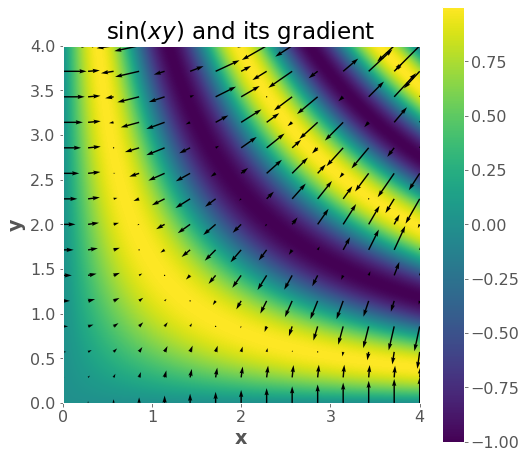
Why is it the direction of fastest increase?#
why go in the gradient direction instead of the \(x_1\) direction, since that first component has the biggest partial derivative? Doesn’t it seem wasteful to go partly in those other directions?
First, a proof that the gradient is the best direction. Let’s say we are at position \(x\) and we move by an infinitesimal (i.e., extremely tiny) vector \(v\), which has components \(v_1, v_2, \ldots, v_d\). The change in \(f\) from moving from \(x\) to \(x+v\) is \(\frac{\partial f}{\partial x_1} v_1 + \frac{\partial f}{\partial x_2} v_2 + \ldots + \frac{\partial f}{\partial x_d} v_d\), where all the partial derivatives are evaluated at \(x\) (this is related to the “total derivative”). In other words, the change in \(f\) is the dot product \(\nabla f \cdot v\). So now the question is, what vector \(v\) of fixed length maximizes \(\nabla f \cdot v\)? The answer is a vector that points in the same direction as \(\nabla f\). (That’s a property of the dot product, and is evident by the definition: \(a \cdot b = \| a \| \| b \| \cos(\theta)\). Since \(\| \nabla f \|\) and \(\| v \|\) are fixed in our case, to maximize this we want to maximize \(\cos(\theta)\), which means we want \(\cos(\theta)=1\), meaning \(\theta=0\), or the angle between the vectors is \(0\)).
Second, the intuition. I think the “paradox” comes from over-privileging the coordinate axes. They are not special in any way! For example, if you rotate the coordinate system by 45 degrees, the direction of steepest ascent should also rotate by 45 degrees. Under the suggested system, this would not happen. Why? Well, there is always going to be one element of the gradient that is largest. Does that mean the direction of steepest ascent is always one of the coordinate axis directions? No. That doesn’t make sense and also fails the “rotate by 45 degrees test” because the direction will have rotated by 0, 90, 180, or 270 degrees.
Images as 3D surfaces#
Show code cell source
# Load an example image from skimage
coffee = data.coffee()
image = rgb2gray(coffee)

# Apply a Gaussian filter to smooth the image
smoothed_image = gaussian(image, sigma=7)

# Create a meshgrid for the image coordinates
x = np.arange(image.shape[1])
y = np.arange(image.shape[0])
x, y = np.meshgrid(x, y)

# Plot the original and smoothed images side by side with the 3D surface
fig = plt.figure(figsize=(14, 6))

# Plot the original 2D image
ax1 = fig.add_subplot(141)
ax1.imshow(image, cmap='gray')
ax1.set_title('Original 2D Image')
ax1.axis('off')

# Plot the smoothed 3D surface
ax2 = fig.add_subplot(142, projection='3d')
ax2.plot_surface(x, y, smoothed_image[:,::-1], cmap='gray')
ax2.view_init(elev=90, azim=90)
ax2.axis('off')

ax3 = fig.add_subplot(143, projection='3d')
ax3.plot_surface(x, y, smoothed_image[:,::-1], cmap='gray')
ax3.view_init(elev=80, azim=90)
ax3.axis('off')

ax4 = fig.add_subplot(144, projection='3d')
ax4.plot_surface(x, y, smoothed_image[:,::-1], cmap='gray')
ax4.view_init(elev=60, azim=90)
ax4.axis('off')

plt.show()

Matrix Differentiation#
Randal J. Barnes, Department of Civil Engineering, University of Minnesota. Minneapolis, Minnesota, USA
Introduction#
Throughout this presentation I have chosen to use a symbolic matrix notation. This choice was not made lightly. I am a strong advocate of index notation, when appropriate. For example, index notation greatly simplifies the presentation and manipulation of differential geometry. As a rule-of-thumb, if your work is going to primarily involve differentiation with respect to the spatial coordinates, then index notation is almost surely the appropriate choice.
In the present case, however, I will be manipulating large systems of equations in which the matrix calculus is relatively simply while the matrix algebra and matrix arithmetic is messy and more involved. Thus, I have chosen to use symbolic notation.
Notation and Nomenclature#
Definition 1. Let \({a}_{{i j}} \in \mathbb{R}, {i}=1,2, \ldots, {m}, {j}=1,2, \ldots, {n}\). Then the ordered rectangular array
is said to be a real matrix of dimension \({m} \times {n}\). When writing a matrix I will occasionally write down its typical element as well as its dimension. Thus,
denotes a matrix with \(m\) rows and \(n\) columns, whose typical element is \(a_{i j}\). Note, the first subscript locates the row in which the typical element lies while the second subscript locates the column. For example, \({a}_{{j k}}\) denotes the element lying in the \({j}^{th}\) row and \(k^{th}\) column of the matrix \(\mathbf{A}\).
Definition 2. A vector is a matrix with only one column. Thus, all vectors are inherently column vectors.
Convention 1
Multi-column matrices are denoted by boldface uppercase letters: for example, \(\mathbf{A}, \mathbf{B}, \mathbf{X}\). Vectors (single-column matrices) are denoted by boldfaced lowercase letters: for example, \(\mathbf{a}, \mathbf{b}, \mathbf{x}\). I will attempt to use letters from the beginning of the alphabet to designate known matrices, and letters from the end of the alphabet for unknown or variable matrices.
Convention 2
When it is useful to explicitly attach the matrix dimensions to the symbolic notation, I will use an underscript. For example, \(\underset{m \times n}{\mathbf{A}}\), indicates a known, multi-column matrix with \(m\) rows and \(n\) columns.
A superscript \({ }^{\top}\) denotes the matrix transpose operation; for example, \(\mathbf{A}^{\top}\) denotes the transpose of \(\mathbf{A}\). Similarly, if \(\mathbf{A}\) has an inverse it will be denoted by \(\mathbf{A}^{-1}\). The determinant of \(\mathbf{A}\) will be denoted by either \(|\mathbf{A}|\) or \(\operatorname{det}(\mathbf{A})\). Similarly, the \(\operatorname{rank}\) of a matrix \(\mathbf{A}\) is denoted by \(\operatorname{rank}(\mathbf{A})\). An identity matrix will be denoted by \(I\), and \(\mathbf{0}\) will denote a null matrix.
Matrix Multiplication#
Definition 3. Let \(\mathbf{A}\) be \({m} \times {n}\), and \(\mathbf{B}\) be \({n} \times p\), and let the product \(\mathbf{A B}\) be
then \(\mathbf{C}\) is a \({m} \times p\) matrix, with element \(({i}, {j})\) given by
for all \(i=1,2, \ldots, m, \quad j=1,2, \ldots, p\).
Proposition 1. Let \(\mathbf{A}\) be \({m} \times {n}\), and \(\mathbf{x}\) be \({n} \times 1\), then the typical element of the product
is given by
for all \({i}=1,2, \ldots, {m}\). Similarly, let \(\mathbf{y}\) be \(m \times 1\), then the typical element of the product
is given by
for all \(i=1,2, \ldots, n\). Finally, the scalar resulting from the product
is given by
Proof: These are merely direct applications of Definition 3. q.e.d.
Proposition 2. Let \(\mathbf{A}\) be \({m} \times {n}\), and \(\mathbf{B}\) be \({n} \times {p}\), and let the product \(\mathbf{A B}\) be
then
Proof: The typical element of \(\mathbf{C}\) is given by
By definition, the typical element of \(\mathbf{C}^{\top}\), say \({d}_{{i j}}\), is given by
Hence,
q.e.d.
Proposition 3. Let \(\mathbf{A}\) and \(\mathbf{B}\) be \({n} \times {n}\) and invertible matrices. Let the product \(\mathbf{A B}\) be given by
then
Proof:
q.e.d.
Partioned Matrices (Further Reading)#
Frequently, I will find it convenient to deal with partitioned matrices \({ }^{1}\). Such a representation, and the manipulation of this representation, are two of the relative advantages of the symbolic matrix notation.
Definition 4. Let \(\mathbf{A}\) be \(m \times n\) and write
where \(\mathbf{B}\) is \({m}_{1} \times {n}_{1}, \mathbf{E}\) is \({m}_{2} \times {n}_{2}, \mathbf{C}\) is \({m}_{1} \times {n}_{2}, \mathbf{D}\) is \({m}_{2} \times {n}_{1}, {m}_{1}+{m}_{2}={m}\), and \({n}_{1}+{n}_{2}={n}\). The above is said to be a partition of the matrix \(\mathbf{A}\).
Proposition 4. Let \(\mathbf{A}\) be a square, nonsingular matrix of order \(m\). Partition \(\mathbf{A}\) as
so that \(\mathbf{A}_{11}\) is a nonsingular matrix of order \({m}_{1}, \mathbf{A}_{22}\) is a nonsingular matrix of order \({m}_{2}\), and \({m}_{1}+{m}_{2}={m}\). Then
Proof: Direct multiplication of the proposed \(\mathbf{A}^{-1}\) and \(\mathbf{A}\) yields
q.e.d.
Matrix Differentiation#
In the following discussion I will differentiate matrix quantities with respect to the elements of the referenced matrices. Although no new concept is required to carry out such operations, the element-by-element calculations involve cumbersome manipulations and, thus, it is useful to derive the necessary results and have them readily available \({ }^{2}\).
Convention 3
Let
where \(\mathbf{y}\) is an \(m\)-element vector, and \(\mathbf{x}\) is an \(n\)-element vector. The symbol
will denote the \(m \times n\) matrix of first-order partial derivatives of the transformation from \(\mathbf{x}\) to \(\mathbf{y}\). Such a matrix is called the Jacobian matrix of the transformation \(\psi()\).
Notice that if \(\mathbf{x}\) is actually a scalar in Convention 3 then the resulting Jacobian matrix is a \(m \times 1\) matrix; that is, a single column (a vector). On the other hand, if \(\mathbf{y}\) is actually a scalar in Convention 3 then the resulting Jacobian matrix is a \(1 \times {n}\) matrix; that is, a single row (the transpose of a vector).
Proposition 5. Let \(\mathbf{y}=\mathbf{A}\mathbf{x} \), where \(\mathbf{y}\) is \({m} \times 1\), \(\mathbf{x}\) is \({n} \times 1, \mathbf{A}\) is \({m} \times {n}\), and \(\mathbf{A}\) does not depend on \(\mathbf{x}\), then
Proof: Since the \(i\) th element of \(\mathbf{y}\) is given by
it follows that
for all \({i}=1,2, \ldots, {m}, \quad {j}=1,2, \ldots, {n}\). Hence
q.e.d.
Proposition 6. Let \(\mathbf{y}=\mathbf{A x} \), where \(\mathbf{y}\) is \({m} \times 1\), \(\mathbf{x}\) is \({n} \times 1, \mathbf{A}\) is \({m} \times {n}\), and \(\mathbf{A}\) does not depend on \(\mathbf{x}\), as in Proposition 5 . Suppose that \(\mathbf{x}\) is a function of the vector \(\mathbf{z}\), while \(\mathbf{A}\) is independent of \(\mathbf{z}\). Then
Proof: Since the \(i\) th element of \(\mathbf{y}\) is given by
for all \({i}=1,2, \ldots, m\), it follows that
but the right hand side of the above is simply element \(({i}, {j})\) of \(\mathbf{A} \frac{\partial \mathbf{x}}{\partial \mathrm{z}}\). Hence
q.e.d.
Proposition 7. Let the scalar \(\alpha\) be defined by
where \(\mathbf{y}\) is \(\mathrm{m} \times 1, \mathbf{x}\) is \(\mathrm{n} \times 1, \mathbf{A}\) is \(\mathrm{m} \times \mathrm{n}\), and \(\mathbf{A}\) is independent of \(\mathbf{x}\) and \(\mathbf{y}\), then
and
Proof: Define
and note that
Hence, by Proposition 5 we have that
which is the first result. Since \(\alpha\) is a scalar, we can write
and applying Proposition 5 as before we obtain
q.e.d.
Proposition 8. For the special case in which the scalar \(\alpha\) is given by the quadratic form
where \(\mathbf{x}\) is \({n} \times 1\), \(\mathbf{A}\) is \({n} \times {n}\), and \(\mathbf{A}\) does not depend on \(\mathbf{x}\), then
Proof: By definition
Differentiating with respect to the \(k^{th}\) element of \(\mathbf{x}\) we have
for all \(\mathrm{k}=1,2, \ldots, \mathrm{n}\), and consequently,
q.e.d.
Proposition 9. For the special case where \(\mathbf{A}\) is a symmetric matrix and
where \(\mathbf{x}\) is \(\mathrm{n} \times 1, \mathbf{A}\) is \(\mathrm{n} \times \mathrm{n}\), and \(\mathbf{A}\) does not depend on \(\mathbf{x}\), then
Proof: This is an obvious application of Proposition 8. q.e.d.
Further Reading#
Proposition 10. Let the scalar \(\alpha\) be defined by
where \(\mathbf{y}\) is \({n} \times 1\), \(\mathbf{x}\) is \({n} \times 1\), and both \(\mathbf{y}\) and \(\mathbf{x}\) are functions of the vector \(\mathbf{z}\). Then
Proof: We have
Differentiating with respect to the k th element of \(\mathbf{z}\) we have
for all \(\mathrm{k}=1,2, \ldots, \mathrm{n}\), and consequently,
q.e.d.
Proposition 11 Let the scalar \(\alpha\) be defined by
where \(\mathbf{x}\) is \(\mathrm{n} \times 1\), and \(\mathbf{x}\) is a function of the vector \(\mathbf{z}\). Then
Proof: This is an obvious application of Proposition 10. q.e.d. Proposition 12 Let the scalar \(\alpha\) be defined by
where \(\mathbf{y}\) is \(\mathrm{m} \times 1, \mathbf{x}\) is \(\mathrm{n} \times 1, \mathbf{A}\) is \(\mathrm{m} \times {n}\), and both \(\mathbf{y}\) and \(\mathbf{x}\) are functions of the vector \(\mathbf{z}\), while \(\mathbf{A}\) does not depend on \(\mathbf{z}\). Then
Proof: Define
and note that
Applying Propositon 10 we have
Substituting back in for \(\mathbf{w}\) we arrive at
q.e.d.
Proposition 13 Let the scalar \(\alpha\) be defined by the quadratic form
where \(\mathbf{x}\) is \({n} \times 1\), \(\mathbf{A}\) is \({n} \times {n}\), and \(\mathbf{x}\) is a function of the vector \(\mathbf{z}\), while \(\mathbf{A}\) does not depend on \(\mathbf{z}\). Then
Proof: This is an obvious application of Proposition 12. q.e.d. Proposition 14 For the special case where \(\mathbf{A}\) is a symmetric matrix and
where \(\mathbf{x}\) is \({n} \times 1\), \(\mathbf{A}\) is \({n} \times {n}\), and \(\mathbf{x}\) is a function of the vector \(\mathbf{z}\), while \(\mathbf{A}\) does not depend on \(\mathbf{z}\). Then
Proof: This is an obvious application of Proposition 13. q.e.d. Definition 5 Let \(\mathbf{A}\) be a \({m} \times {n}\) matrix whose elements are functions of the scalar parameter \(\alpha\). Then the derivative of the matrix \(\mathbf{A}\) with respect to the scalar parameter \(\alpha\) is the \(m \times n\) matrix of element-by-element derivatives:
Proposition 15 Let A be a nonsingular, \(\mathrm{m} \times \mathrm{m}\) matrix whose elements are functions of the scalar parameter \(\alpha\). Then
Proof: Start with the definition of the inverse
and differentiate, yielding
rearranging the terms yields
q.e.d.
References#
Dhrymes, Phoebus J., 1978, Mathematics for Econometrics, Springer-Verlag, New York, 136 pp.
Golub, Gene H., and Charles F. Van Loan, 1983, Matrix Computations, Johns Hopkins University Press, Baltimore, Maryland, 476 pp.
Graybill, Franklin A., 1983, Matrices with Applications in Statistics, 2nd Edition, Wadsworth International Group, Belmont, California, 461 pp .
[1]: Much of the material in this section is extracted directly from Dhrymes (1978, Section 2.7).
[2]: Much of the material in this section is extracted directly from Dhrymes (1978, Section 4.3). The interested reader is directed to this worthy reference to find additional results.