Learning Vector Quantization (LVQ)
Learning Vector Quantization (LVQ)¶

Computer Science Dept, Ferdowsi University of Mashhad
Where this page sits¶
Chapter 13 of Hastie et al. (2009) is about prototype methods: instead of fitting a parametric model, keep a small set of points in feature space and classify by proximity to them. The chapter develops three of them in turn:
| method | prototypes are placed using | supervision |
|---|---|---|
| K-means clustering (§13.2.1) | the geometry of each class separately | labels used only after clustering |
| LVQ (§13.2.2) | the geometry of all classes at once | labels used during training |
| Gaussian mixtures (§13.2.3) | a density model per class | soft, likelihood based |
This page follows §13.2.2. It states the classifier, gives the algorithm (Algorithm 13.1 of the book), implements it from scratch in a few lines of NumPy, and compares the prototypes it produces with the ones K-means produces on the same data — the comparison the book makes in Figure 13.1.
What you should be able to do at the end¶
state the nearest-prototype classifier and say what the prototypes are;
write the LVQ1 update rule from memory and explain the sign of the two branches (attract / repel);
explain why the learning rate has to go to zero, and why K-means prototypes are a good starting point;
describe how K-means prototypes differ from LVQ prototypes in a picture, and why the difference is a consequence of who “has a say” in placing them;
name the price the method pays for being defined by an algorithm rather than by the minimisation of a criterion.
1. The nearest-prototype classifier¶
Fix a number of prototypes per class, R, and let K be the number of classes.
Training produces K*R prototypes m_1, ..., m_{K*R}, each carrying a class
label c_j. A new point x is classified by the label of the closest
prototype:
Two things make this attractive for teaching and for practice: the decision boundary can be arbitrarily curved (it is a union of Voronoi cells), and the model is just a list of points, so it can be drawn, stored and explained. Everything difficult is in the question where to put the prototypes, and that is where the methods differ.
The book standardises the features to mean 0 and variance 1 before using Euclidean distance (p. 461), and so do we.
2. The problem that LVQ is answering¶
The straightforward recipe of §13.2.1 is: cluster the training data of each
class separately with R centres, keep all centres, and classify by the
nearest one. It works, and it has a visible weakness that the book points out
(p. 462):
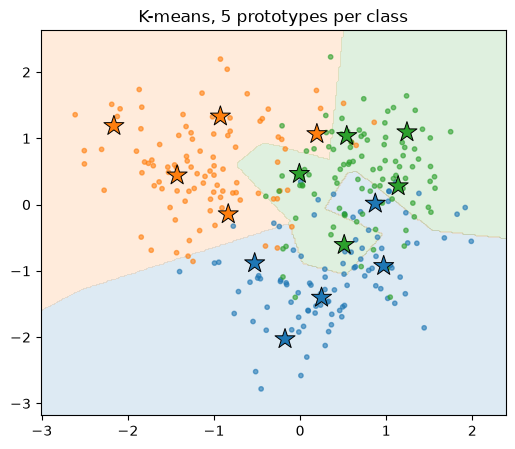
… prototypes are near the class boundaries, leading to potential misclassification errors for points near these boundaries. This results from an obvious shortcoming with this method: for each class, the other classes do not have a say in the positioning of the prototypes for that class.
A prototype computed inside one class has no idea that another class is nearby, so it is happy to sit on the frontier. LVQ fixes exactly this: the update rule sees the label of the training point and the label of the nearest prototype, so a prototype that is winning points of the wrong class is pushed away.
3. A simulated three-class problem¶
To see the difference we need data where the classes touch, since with well-separated classes every method looks the same. We use the simulation of ESL §2.3.3 — the one behind Figure 13.1 — with three classes instead of two:
three classes, two features;
each class has 10 means, drawn from a normal distribution centred at a class-specific location —
(1.5,0),(0,1.5)and(1.5,1.5)— with covarianceI/4;each observation is generated by picking one of the ten means at random (probability
1/10) and adding Gaussian noise with covarianceI/5.
This is the “model somewhere between the two scenarios” of p. 16: the classes
are neither linearly separable nor far apart, and the Bayes boundary is
genuinely curved. The spread of the ten means (I/4) is narrower than the book’s
I, which keeps the problem hard without making it hopeless: even a good rule
errs on a sizeable fraction of the points, but nothing like the two-in-three of
a coin toss among three classes.
Source
import numpy as np
import matplotlib.pyplot as plt
from sklearn.cluster import KMeans
from sklearn.datasets import load_iris
from sklearn.model_selection import train_test_split
from skimage import data
from skimage.color import rgb2gray
from skimage.util import view_as_blocks

%matplotlib inline
COLORS = np.array(["tab:blue", "tab:orange", "tab:green"])
Source
def make_mixture(n_per_class=100, n_means=10, seed=0):
    """ESL section 2.3.3 simulation, extended to three classes (Figure 13.1).

    Each class owns ten means, drawn around that class's own centre with
    covariance I/4; every observation is one mean plus N(0, I/5) noise.
    """
    rng = np.random.default_rng(seed)
    centres = np.array([[1.5, 0.0], [0.0, 1.5], [1.5, 1.5]])   # one per class
    X, y = [], []
    for k in range(3):
        means = centres[k] + rng.normal(scale=0.5, size=(n_means, 2))  # 10 means
        pick = rng.integers(0, n_means, size=n_per_class)      # one mean per observation
        noise = rng.normal(scale=np.sqrt(1 / 5), size=(n_per_class, 2))
        X.append(means[pick] + noise)
        y.append(np.full(n_per_class, k))
    return np.vstack(X), np.concatenate(y)


def standardize(X_train, *others):
    """Standardise with the statistics of the training set only."""
    mu, sd = X_train.mean(axis=0), X_train.std(axis=0)
    return [(Z - mu) / sd for Z in (X_train, *others)]


X_train, y_train = make_mixture(seed=0)
X_test, y_test = make_mixture(seed=1)          # same distribution, new sample
X_train, X_test = standardize(X_train, X_test)  # scale with training statistics
X_train.shape, np.bincount(y_train)
((300, 2), array([100, 100, 100]))Source
fig, ax = plt.subplots(figsize=(6, 5))
for k in range(3):
    ax.scatter(X_train[y_train == k, 0], X_train[y_train == k, 1],
               s=14, color=COLORS[k], alpha=0.7, label=f"class {k}")
ax.set_title("the simulated problem: three overlapping classes")
ax.legend();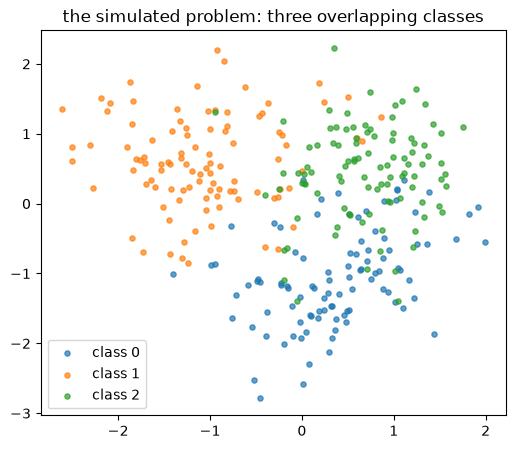
4. K-means prototypes (the starting point)¶
R = 5 prototypes per class, produced by clustering the points of each class
separately. Every prototype inherits the label of the class it was computed in.
Source
def kmeans_prototypes(X, y, R=5, seed=0):
    """R centres per class: ESL section 13.2.1."""
    protos, pclass = [], []
    for k in np.unique(y):
        km = KMeans(n_clusters=R, n_init=10, random_state=seed).fit(X[y == k])
        protos.append(km.cluster_centers_)
        pclass.append(np.full(R, k))
    return np.vstack(protos), np.concatenate(pclass)


def predict(X, protos, pclass):
    """Nearest-prototype classifier: the label of the closest prototype."""
    d = ((X[:, None, :] - protos[None, :, :]) ** 2).sum(axis=2)
    return pclass[d.argmin(axis=1)]


def plot_regions(ax, protos, pclass, X, y, title):
    pad = 0.4
    xs = np.linspace(X[:, 0].min() - pad, X[:, 0].max() + pad, 300)
    ys = np.linspace(X[:, 1].min() - pad, X[:, 1].max() + pad, 300)
    xx, yy = np.meshgrid(xs, ys)
    zz = predict(np.c_[xx.ravel(), yy.ravel()], protos, pclass).reshape(xx.shape)
    ax.contourf(xx, yy, zz, levels=[-0.5, 0.5, 1.5, 2.5], colors=COLORS, alpha=0.15)
    ax.scatter(X[:, 0], X[:, 1], c=COLORS[y], s=10, alpha=0.6)
    ax.scatter(protos[:, 0], protos[:, 1], c=COLORS[pclass], marker="*",
               s=230, edgecolor="black", linewidth=0.7)
    ax.set_title(title)


protos_km, class_km = kmeans_prototypes(X_train, y_train, R=5)
print("prototypes:", protos_km.shape)
fig, ax = plt.subplots(figsize=(6, 5))
plot_regions(ax, protos_km, class_km, X_train, y_train, "K-means, 5 prototypes per class");
prototypes: (15, 2)
5. The LVQ algorithm¶
Algorithm 13.1 (Learning Vector Quantization — LVQ), as printed in Hastie et al. (2009), p. 462
Choose
Rinitial prototypes for each classm_1^(k), ..., m_R^(k),k = 1..K— for example by samplingRtraining points at random from each class, or by running K-means on each class.Sample a training point
x_iat random (with replacement), and let(j,k)index the closest prototypem_j^(k)tox_i.(a) If
g_i = k— the same class — move the prototype towards the training point:(b) If
g_i != k— a different class — move the prototype away from the training point:
Repeat step 2, decreasing the learning rate
εwith each iteration towards zero.
Three remarks that the book makes next:
LVQ is an online algorithm: observations arrive one at a time, and each one updates a single prototype.
The decay of
εmust obey the stochastic-approximation conditions of §11.4 (ε_t -> 0,sum ε_t = infinity,sum ε_t^2 < infinity); a schedule such asε_t = ε_0 / (1 + t)satisfies them.The procedure above is LVQ1; variants (LVQ2, LVQ3) exist. A drawback of the whole family is that they are defined by an algorithm rather than by the minimisation of a fixed criterion, which makes their properties harder to analyse. Newer cost-function-based versions (generalised LVQ) were invented precisely to repair this.
The book also uses the K-means solution as the starting values, and gets the result shown in its Figure 13.1 (lower panel): the prototypes have moved away from the decision boundaries and away from prototypes of competing classes.
Source
def lvq1(X, y, protos, pclass, epochs=150, eps0=0.1, seed=0):
    """Online LVQ1, as Algorithm 13.1 of ESL."""
    m, c = protos.copy(), pclass.copy()
    rng = np.random.default_rng(seed)
    errors = []

    for epoch in range(epochs):
        eps = eps0 / (1.0 + epoch)              # step 3: eps -> 0 as 1/t
        for i in rng.permutation(len(X)):       # step 2: sample a point at random
            x = X[i]
            j = ((m - x) ** 2).sum(axis=1).argmin()   # the closest prototype
            if c[j] == y[i]:
                m[j] += eps * (x - m[j])        # (a) same class    -> attract
            else:
                m[j] -= eps * (x - m[j])        # (b) other class   -> repel
        errors.append((predict(X, m, c) != y).mean())

    return m, c, errors
Source
protos_lvq, class_lvq, errors = lvq1(X_train, y_train, protos_km, class_km)

fig, axes = plt.subplots(1, 2, figsize=(12, 5))
plot_regions(axes[0], protos_km, class_km, X_train, y_train,
             "K-means prototypes (before LVQ)")
plot_regions(axes[1], protos_lvq, class_lvq, X_train, y_train,
             "after LVQ1: prototypes leave the boundary")
plt.tight_layout()
print(f"training error before LVQ: {(predict(X_train, protos_km, class_km) != y_train).mean():.3f}")
print(f"training error after  LVQ: {(predict(X_train, protos_lvq, class_lvq) != y_train).mean():.3f}")
training error before LVQ: 0.240
training error after LVQ: 0.170
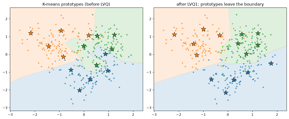
Look at the stars in the two panels. In the left one several prototypes sit inside the territory of another colour; in the right one they have been pulled into their own region and pushed away from the frontier. That is the whole effect of the sign in step 2, repeated a few thousand times.
Source
fig, ax = plt.subplots(figsize=(7, 4))
ax.plot(errors, color="tab:blue")
ax.set_xlabel("epoch")
ax.set_ylabel("training error of the nearest-prototype rule")
ax.set_title("LVQ1 on the simulated problem")
ax.grid(alpha=0.3);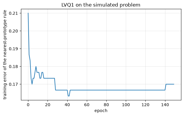
Measuring “away from the boundary”¶
A single number makes the claim checkable: for every prototype, compute the distance to the nearest prototype of a different class, and take the median. LVQ should increase it, because a prototype that is close to an enemy is the one the repel step keeps hitting.
Source
def median_gap_to_enemy(protos, pclass):
    d = np.sqrt(((protos[:, None, :] - protos[None, :, :]) ** 2).sum(axis=2))
    d[pclass[:, None] == pclass[None, :]] = np.inf      # ignore same-class pairs
    return np.median(d.min(axis=1))


print(f"median distance to the nearest other-class prototype")
print(f"  before LVQ : {median_gap_to_enemy(protos_km, class_km):.3f}")
print(f"  after  LVQ : {median_gap_to_enemy(protos_lvq, class_lvq):.3f}")
median distance to the nearest other-class prototype
before LVQ : 0.800
after LVQ : 1.493
6. Does it help on unseen data?¶
Prototypes that leave the training points can also leave the useful ones, so the training error alone proves nothing. The honest test is a fresh sample from the same distribution, which we generated with a different seed.
Source
rows = []
for name, protos, pclass in [
    ("K-means prototypes", protos_km, class_km),
    ("LVQ1 prototypes", protos_lvq, class_lvq),
]:
    rows.append((name, (predict(X_train, protos, pclass) != y_train).mean(),
                 (predict(X_test, protos, pclass) != y_test).mean()))

print(f"{'prototypes':22s}{'train error':>13s}{'test error':>12s}")
for name, tr, te in rows:
    print(f"{name:22s}{tr:13.3f}{te:12.3f}")
prototypes train error test error
K-means prototypes 0.240 0.277
LVQ1 prototypes 0.170 0.227
The numbers move by a few points, in the direction the book describes, and the size of the improvement is itself part of the lesson: LVQ is a cheap, local repair of a K-means solution, not a different model class. Where the classes are well separated it changes almost nothing; where they overlap, it redraws the frontier.
7. Practical notes¶
Initialisation. ESL starts from the K-means solution, and so should anyone in practice: starting from random training points leaves far more work for the online updates. The next cell shows the difference on the same data.
Learning rate. ε_0 sets how far a prototype moves on one observation;
epochs sets how long the schedule runs. Too large and the prototypes oscillate,
too small and they never arrive. ε_t = ε_0/(1+t) is a safe default.
R, the number of prototypes per class. More prototypes give a finer
boundary and a larger model; R = 1 reduces LVQ to a nearest-centroid
classifier, and the update rule to a perceptron-like correction of the centroids.
Feature scaling. Euclidean distance is meaningless without it; standardise as ESL does, with the training statistics.
Sampling with replacement. Step 2 draws a random training point every time, not a pass over a shuffled list, so classes with more points are seen more often. For imbalanced data that is a bias worth knowing about.
Source
def random_prototypes(X, y, R=5, seed=0):
    rng = np.random.default_rng(seed)
    protos, pclass = [], []
    for k in np.unique(y):
        idx = rng.choice(np.flatnonzero(y == k), size=R, replace=False)
        protos.append(X[idx])
        pclass.append(np.full(R, k))
    return np.vstack(protos), np.concatenate(pclass)


rng_protos, rng_class = random_prototypes(X_train, y_train, R=5)
trials = [
    ("random start, eps0=0.1", rng_protos, rng_class, 0.1),
    ("k-means start, eps0=0.1", protos_km, class_km, 0.1),
    ("k-means start, eps0=0.5", protos_km, class_km, 0.5),
]
for name, p0, c0, eps0 in trials:
    m, c, _ = lvq1(X_train, y_train, p0, c0, eps0=eps0)
    print(f"{name:26s} test error = {(predict(X_test, m, c) != y_test).mean():.3f}")
random start, eps0=0.1 test error = 0.250
k-means start, eps0=0.1 test error = 0.227
k-means start, eps0=0.5 test error = 0.207
8. On real data: the iris flowers¶
Four features, three classes, R = 3 prototypes per class. With R equal to the
class count and well-behaved data the prototypes end up near the class means, so
LVQ has little to repair — which is exactly why the simulated problem above was
needed to see the effect.
Source
iris = load_iris()
Xi, yi = iris.data, iris.target
Xi_train, Xi_test, yi_train, yi_test = train_test_split(
    Xi, yi, test_size=0.3, random_state=0, stratify=yi)
Xi_train, Xi_test = standardize(Xi_train, Xi_test)

p0, c0 = kmeans_prototypes(Xi_train, yi_train, R=3)
m_i, c_i, _ = lvq1(Xi_train, yi_train, p0, c0, epochs=100)

centroids = np.vstack([Xi_train[yi_train == k].mean(axis=0) for k in range(3)])
for name, protos, pclass in [
    ("nearest centroid (R=1)", centroids, np.arange(3)),
    ("K-means prototypes (R=3)", p0, c0),
    ("LVQ1 prototypes (R=3)", m_i, c_i),
]:
    te = (predict(Xi_test, protos, pclass) != yi_test).mean()
    print(f"{name:26s} test error = {te:.3f}")
nearest centroid (R=1) test error = 0.244
K-means prototypes (R=3) test error = 0.000
LVQ1 prototypes (R=3) test error = 0.000
9. Where the name comes from¶
“Quantization” is the older idea behind the method: replace a vector by the
index of the nearest prototype and store only that index. With K prototypes
each index costs log2(K) bits instead of the bits of a whole vector, so the
prototype set becomes a codebook and the method becomes lossy compression.
The name survives in the title of LVQ, but the compression application is a different lesson: it uses K-means with no labels at all and is measured in bits and decibels rather than in error rates. It therefore has a page of its own:
Vector Quantization and Image Compression — ESL §14.3.9, with the rate/distortion trade-off measured on a test image.
Summary¶
A prototype method classifies by the label of the closest prototype;
K*Rprototypes encode a curved decision boundary.Clustering each class on its own (§13.2.1) puts prototypes where that class is dense, with no regard for the others, so they drift onto the boundaries — the shortcoming the book names explicitly.
LVQ (§13.2.2) is online and label-aware: the point attracts the closest prototype of its own class and repels the closest prototype of another class, with a step
εthat decays to zero.This is LVQ1; LVQ2, LVQ3 extend it, and the family has no fixed objective function — that is the method’s price.
Starting from the K-means prototypes (ESL’s choice) is far better than starting from random points, and the effect of LVQ is a local repair of the boundary.
The same “nearest prototype + store the index” idea, applied to image blocks, is vector quantization: the origin of the name, and a compression method with a page of its own.
Exercises¶
Set
R = 1and run LVQ on the simulated data. What does the update rule become, and why does the boundary stay almost straight?Replace the schedule
ε_t = ε_0/(1+t)by a constantε = 0.1. Plot the training error against the epoch: what do you see, and which of the three stochastic-approximation conditions is violated?Use
R = 2, 5, 10, 20prototypes per class and plot the test error. Where does the curve flatten, and what is the cost per prototype?Attract-only variant: delete the repel branch and train from the K-means start. Explain the result in terms of the book’s sentence about who has a say in the placement of prototypes.
Calculate the Bayes error of the simulated problem analytically (or estimate it with a very large 1-NN model) and compare it with the errors of the two prototype sets.
For the compression experiment, try
bs = 2andbs = 8with the same number of bits per pixel. Which block size gives the better picture, and why is tile structure visible in the reconstruction?
Sources¶
The method, its algorithm (Algorithm 13.1) and the simulated example: §13.2.2 and §13.2 of Hastie et al. (2009) (2nd edition, pp. 461–463); the compression application is on its own page (§14.3.9 of the same book). Figures on this page are generated by the code above, reproducing the comparison of ESL Figure 13.1.
Kohonen’s original LVQ papers are the references given there; the GLVQ reformulation is the cost-function-based repair of the “no fixed criterion” objection.
sklearn.cluster.KMeansdocumentation for the implementation used to build the initial prototypes.
- Hastie, T., Tibshirani, R., & Friedman, J. (2009). The Elements of Statistical Learning: Data Mining, Inference, and Prediction (2nd ed.). Springer. 10.1007/978-0-387-84858-7