K-Medoids

Where this page sits¶
Section 14.3.10 of Hastie et al. (2009) (pp. 515-518) repairs the two restrictions that K-means acquires from its objective: it needs attribute values to average, and its squared Euclidean distance gives the largest distances the largest influence, which makes it fragile against outliers.
The repair is small. Of the two steps of K-means, only one uses the squared distance: replacing each cluster by its mean. If that step is replaced by “replace each cluster by one of its own observations”, any dissimilarity at all becomes usable - including the proximity matrices of the previous page, where no averaging is possible.
What you should be able to do at the end¶
write Algorithm 14.2 and point at the one line that differs from K-means;
say why K-medoids accepts an arbitrary dissimilarity matrix and K-means does not;
count the cost: instead of per cluster, and say when that is worth paying;
read the country-dissimilarity example, including its reordered matrix and its MDS display.
1. The one step that assumes squared distance¶
K-means minimises the within-cluster scatter, and it does so by alternating two steps: assign every point to the nearest centre, then move every centre to the mean of its points. The second step is optimal only for squared Euclidean distance, because (14.32) of the book says
which is the mean and nothing else. Change the distance and the mean is no longer the best representative; replace the distance by a table of dissimilarities and the mean is not even defined.
The general statement of the method keeps the criterion and drops the shortcut. Centre of cluster is chosen to minimise the total dissimilarity to the cluster’s own members:
For a general that minimisation is a search over the cluster’s own observations, and the minimiser is an observation - a medoid. It is not a new point, it is the most central existing point, which is why the medoid can be shown to a domain expert and why it exists for categorical data.
2. Algorithm 14.2¶
As printed in Hastie et al. (2009), p. 516:
For a given cluster assignment , find the observation in each cluster that minimises the total distance to the other points of that cluster:
and set for .
Given the centres, assign every observation to the nearest one:
Iterate until the assignments stop changing.
The price is visible in the two line counts. Step 2 costs , as in K-means. Step 1 costs per cluster instead of , because every member is compared with every other member; over a full run that is the difference between linear and quadratic work in each cluster. The book says it plainly: K-medoids is far more computationally intensive than K-means.
Even so, Algorithm 14.2 is a heuristic for the combinatorial problem (14.38). Kaufman and Rousseeuw’s PAM improves on it by trying to exchange a current medoid with a non-medoid and keeping the exchange that reduces the criterion most, repeated until no exchange helps; Massart et al. give a branch-and-bound method that finds the global optimum for very small data sets.
Below is Algorithm 14.2 as written, with many random starts because - as on the families page - the criterion has local minima.
import numpy as np
import matplotlib.pyplot as plt

names = ["BEL", "BRA", "CHI", "CUB", "EGY", "FRA",
         "IND", "ISR", "USA", "USS", "YUG", "ZAI"]
lower = {
    "BRA": [5.58],
    "CHI": [7.00, 6.50],
    "CUB": [7.08, 7.00, 3.83],
    "EGY": [4.83, 5.08, 8.17, 5.83],
    "FRA": [2.17, 5.75, 6.67, 6.92, 4.92],
    "IND": [6.42, 5.00, 5.58, 6.00, 4.67, 6.42],
    "ISR": [3.42, 5.50, 6.42, 6.42, 5.00, 3.92, 6.17],
    "USA": [2.50, 4.92, 6.25, 7.33, 4.50, 2.25, 6.33, 2.75],
    "USS": [6.08, 6.67, 4.25, 2.67, 6.00, 6.17, 6.17, 6.92, 6.17],
    "YUG": [5.25, 6.83, 4.50, 3.75, 5.75, 5.42, 6.08, 5.83, 6.67, 3.67],
    "ZAI": [4.75, 3.00, 6.08, 6.67, 5.00, 5.58, 4.83, 6.17, 5.67, 6.50, 6.92],
}

n = len(names)
D = np.zeros((n, n))
for i, country in enumerate(names[1:], start=1):
    for j, value in enumerate(lower[country]):
        D[i, j] = D[j, i] = value


def k_medoids(D, K, n_starts=60, seed=0, max_iter=100):
    """Algorithm 14.2 with random starts; keeps the best solution found."""
    rng = np.random.default_rng(seed)
    N = len(D)
    best = None
    for _ in range(n_starts):
        med = rng.choice(N, K, replace=False)
        for _ in range(max_iter):
            lab = D[:, med].argmin(axis=1)
            new = med.copy()
            for k in range(K):
                members = np.where(lab == k)[0]
                if len(members) == 0:
                    continue
                sub = D[np.ix_(members, members)]
                new[k] = members[sub.sum(axis=1).argmin()]
            new = np.sort(new)
            if np.array_equal(new, med):
                break
            med = new
        lab = D[:, med].argmin(axis=1)
        if len(np.unique(med)) < K:            # two clusters chose the same medoid
            continue
        cost = D[np.arange(N), med[lab]].sum()
        if best is None or cost < best[0]:
            best = (cost, med.copy(), lab.copy())
    return best


cost, medoids, labels = k_medoids(D, K=3)
print("criterion (sum of distances to the medoid):", round(cost, 2))
print("medoids:", [names[i] for i in medoids])
for k in range(3):
    members = [names[i] for i in np.where(labels == k)[0]]
    print(f"  cluster {k}: {members}")
criterion (sum of distances to the medoid): 30.08
medoids: ['CUB', 'USA', 'ZAI']
cluster 0: ['CHI', 'CUB', 'USS', 'YUG']
cluster 1: ['BEL', 'EGY', 'FRA', 'ISR', 'USA']
cluster 2: ['BRA', 'IND', 'ZAI']
Three groups come out, and they are the ones a reader of the 1990 survey would expect: a western group around the United States, France, Israel and Belgium, a second around Cuba and the USSR together with China and Yugoslavia, and a third of Brazil, India and Zaire. Egypt joins the western group, but the MDS display below shows why the book singles it out: it sits about halfway between two groups, so its assignment is a matter of a few tenths of a dissimilarity unit.
The left panel of Figure 14.10 in the book is the dissimilarity matrix with its rows and columns reordered by cluster, so that the blocks appear on the diagonal.
order = np.argsort(labels, kind="stable")
fig, ax = plt.subplots(figsize=(5.5, 5))
im = ax.imshow(D[np.ix_(order, order)], cmap="magma_r")
ax.set_xticks(range(n))
ax.set_xticklabels([names[i] for i in order], rotation=90)
ax.set_yticks(range(n))
ax.set_yticklabels([names[i] for i in order])
ax.set_title("Dissimilarities reordered by the 3-medoid clustering")
fig.colorbar(im, ax=ax, label="dissimilarity")
plt.show()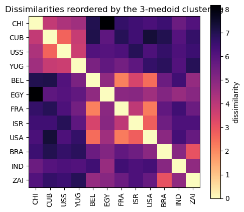
The three dark blocks on the diagonal are the three clusters: within a block the entries are small, between blocks they are large. This picture is the clustering, and it is worth more than a list of labels, because the off-diagonal entries show how close the groups are to each other - Brazil’s block is far from both others, the western and the ex-Soviet blocks are not so far apart.
3. The same clustering in two dimensions¶
Distances cannot be drawn, but a two-dimensional multidimensional scaling of them can: find points whose pairwise Euclidean distances are as close as possible to the given dissimilarities. The right panel of Figure 14.10 is this plot; it is a diagnostic and not a proof, since the two coordinates are fitted and can be rotated or reflected arbitrarily.
from sklearn.manifold import MDS

mds = MDS(n_components=2, dissimilarity="precomputed", random_state=0, n_init=10)
Y = mds.fit_transform(D)

colours = ["tab:blue", "tab:orange", "tab:green"]
fig, ax = plt.subplots(figsize=(6, 5))
for k in range(3):
    ax.scatter(Y[labels == k, 0], Y[labels == k, 1],
               s=60, color=colours[k], label=f"cluster {k + 1}")
for i, name in enumerate(names):
    ax.annotate(name, (Y[i, 0], Y[i, 1]), xytext=(4, 4), textcoords="offset points")
ax.set_xlabel("first MDS coordinate")
ax.set_ylabel("second MDS coordinate")
ax.legend()
ax.set_title("Metric MDS of the country dissimilarities")
plt.show()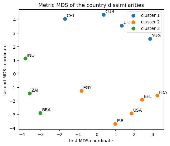
4. Why not just use K-means on attribute data?¶
With attribute data both methods apply, so the choice is about the loss. Squared Euclidean distance multiplies a large difference by itself, so a handful of distant points can pull a mean far from the bulk of its cluster; a sum of distances, which is what the medoid minimises, treats one large deviation linearly. The experiment below is the smallest version of the effect: one compact cloud of 40 points, and three points far away. The mean of the forty-three points is pulled towards the stragglers; the medoid is one of the observations and cannot move.
rng = np.random.default_rng(5)
cloud = rng.normal((0.0, 0.0), 0.6, size=(40, 2))
stragglers = np.array([[6.0, 5.0], [7.0, 6.0], [5.5, 7.0]])
P = np.vstack([cloud, stragglers])

P_dist = np.sqrt(((P[:, None, :] - P[None, :, :]) ** 2).sum(-1))
mean_of_P = P.mean(axis=0)
medoid_of_P = P[P_dist.sum(axis=1).argmin()]

print("true centre of the cloud     : (0.00, 0.00)")
print("mean of all 43 points        :", np.round(mean_of_P, 2))
print("medoid of all 43 points      :", medoid_of_P)
print(f"distance from the true centre: mean {np.linalg.norm(mean_of_P):.2f}, "
      f"medoid {np.linalg.norm(medoid_of_P):.2f}")
true centre of the cloud : (0.00, 0.00)
mean of all 43 points : [0.42 0.24]
medoid of all 43 points : [-0.02273144 -0.18260265]
distance from the true centre: mean 0.48, medoid 0.18
The distance in the last line is the whole argument. A centroid is a computed position: it can land between two groups, or outside the data altogether, when the cluster contains a point that does not belong to it. A medoid is always one of the observations, so its worst case is “a real member of the cluster that is not very central”, never “a place where nothing was measured”. On clean attribute data the two methods usually agree, so the reason to prefer K-medoids is not accuracy - it is that its answer is robust to the kind of point that is common in real data (a mis-recorded measurement, a heavy tail, a survey respondent who answered carelessly).
The cost is real, so the practical rule is:
attribute data, squared loss acceptable, many points - K-means;
only dissimilarities available (the country survey, a confusion matrix, a string-edit table) - K-medoids, which is the only option;
attribute data with outliers, or small and moderate - K-medoids if the quadratic step is affordable, otherwise K-means on medians or a trimmed variant.
Summary¶
K-medoids is K-means with the mean replaced by a member of the cluster, which removes both the squared-distance assumption and the need for coordinates.
Algorithm 14.2 alternates (14.35) and (14.36); only step 1 is new, and it costs per cluster.
The criterion (14.38) still has local minima, so multiple starts are still necessary; PAM exchanges medoids, and branch-and-bound can solve tiny instances exactly.
On the country data the three medoids give three interpretable groups, and the reordered matrix and the MDS plot are the two ways the book displays them.
The reason to use it is robustness and generality, not accuracy on clean attribute data.
Exercises¶
Replace the medoid update by a mean update in
k_medoidsand run it on the country matrix. What fails, and why is that the whole point of the section?Implement the Kaufman-Rousseeuw exchange: from a solution of Algorithm 14.2, try exchanging each medoid with each non-medoid and keep the best exchange. How much does the criterion improve on the country data?
Cluster the countries with and . Which group splits first, and does Egypt move?
Compare the medoids with the clustering you get from the squared dissimilarities . Which clusters change?
Time both methods on the iris data for and for a sample of . How does the ratio of run times grow with ?
K-medoids with the median instead of the medoid of each coordinate is another robust variant. Is it the same algorithm? Give a counterexample if not.
Sources¶
Algorithm 14.2, (14.35)-(14.38), the complexity remark and the country example: §14.3.10 of Hastie et al. (2009), pp. 515-518.
The survey data (Table 14.3) and PAM: Kaufman and Rousseeuw (1990), cited there; the same matrix is used on the proximity matrices page.
Multidimensional scaling is §14.8 of the same book;
sklearn.manifold.MDSimplements the metric version used above.
- Hastie, T., Tibshirani, R., & Friedman, J. (2009). The Elements of Statistical Learning: Data Mining, Inference, and Prediction (2nd ed.). Springer. 10.1007/978-0-387-84858-7