Self-Organizing Maps

Where this page sits¶
Section 14.4 of Hastie et al. (2009) (pp. 528-533) is the last clustering method of the chapter, and the book introduces it in one sentence that is also its definition: a self-organizing map (SOM) is K-means with the prototypes constrained to lie on a one- or two-dimensional manifold in feature space. The constraint is what makes the result a map: the prototypes carry grid coordinates, so every observation can be placed on a two-dimensional display, and neighbouring cells of the display hold similar observations.
Kohonen’s method is older than the machine-learning vocabulary around it, and it is still the standard tool for visualising document collections; WEBSOM, the example the section closes with, is a map of twelve thousand newsgroup articles.
What you should be able to do at the end¶
describe a SOM as a grid of prototypes and write the online update (14.46);
say what the neighbourhood radius and the learning rate do, and how both are scheduled;
write the batch update (14.48) and show that it becomes K-means when the neighbourhood shrinks to one cell;
judge whether the two-dimensional constraint is acceptable on a given data set by comparing reconstruction errors with K-means.
1. The model¶
Fix a grid, say cells, and one prototype per cell. Each prototype carries an integer coordinate pair - its position on the map, not in feature space. The map is a two-dimensional coordinate system, and the prototypes are points of the feature space assigned to cells of it.
The book’s picture is worth keeping: initialise the prototypes in the plane of the first two principal components and think of them as buttons sewn on that plane in a regular pattern. Fitting the SOM bends the plane so that the buttons follow the data. Distances between buttons are measured on the map, not in feature space, and that is the constraint: prototypes that are neighbours on the grid are pulled towards the same observations, so they stay neighbours in feature space.
2. The online algorithm¶
Observations are processed one at a time. Find the closest prototype to in , then move it and its map-neighbours towards :
The neighbourhood always contains the winner itself. The general form weights the step by the map distance,
with decreasing in the map distance - a Gaussian, or the indicator of a disc.
Both schedules in the book go from coarse to fine: the learning rate falls from about 1.0 to 0 over a few thousand iterations, and the radius falls linearly from an initial to 1. Early, large neighbourhoods make the map globally smooth; late, small ones let it fit local structure. This is the same annealing idea as in LVQ, and the same warning applies: the method is defined by its schedule, not by the minimisation of a criterion.
If is small enough that every neighbourhood is a single cell, the spatial connection is lost and the algorithm becomes online K-means: it converges to one of the local minima that K-means also finds. That is the sense in which the SOM is a constrained K-means, and it also tells you how to check the constraint on a given problem:
It is necessarily larger for the SOM than for K-means with the same number of prototypes. If it is much larger, the two-dimensional map is a bad description of the data.
3. A worked example: three clusters on a half sphere¶
The book’s example is 90 points in near the surface of a half sphere of radius 1, in three clusters near , and . The red cluster is deliberately much tighter than the other two, which is what makes the fitted map fold back on itself.
import warnings

import numpy as np
import matplotlib.pyplot as plt

warnings.filterwarnings("ignore", message="KMeans is known to have a memory leak")

rng = np.random.default_rng(0)


def on_sphere(centre, sd, count):
    P = np.asarray(centre, float) + rng.normal(0.0, sd, size=(count, 3))
    return P / np.linalg.norm(P, axis=1, keepdims=True)


red = on_sphere((0, 1, 0), 0.04, 30)      # the tight cluster
green = on_sphere((0, 0, 1), 0.13, 30)
blue = on_sphere((1, 0, 0), 0.13, 30)
X = np.vstack([red, green, blue])
truth = np.repeat([0, 1, 2], 30)
colours = np.array(["tab:red", "tab:green", "tab:blue"])[truth]

fig = plt.figure(figsize=(5.5, 5))
ax = fig.add_subplot(111, projection="3d")
ax.scatter(X[:, 0], X[:, 1], X[:, 2], c=colours, s=14)
ax.set_title("90 points near a half sphere, in three clusters")
plt.show()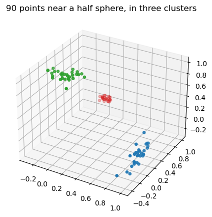
The prototypes are initialised on the first two principal components, spread over the extent of the data - the “buttons sewn on the plane” of the section.
q1 = q2 = 5                       # a 5 x 5 grid: 25 prototypes
mu = X.mean(axis=0)
U, S, Vt = np.linalg.svd(X - mu, full_matrices=False)
scores = (X - mu) @ Vt[:2].T

a1 = np.linspace(scores[:, 0].min(), scores[:, 0].max(), q1)
a2 = np.linspace(scores[:, 1].min(), scores[:, 1].max(), q2)
grid = np.array([[u, v] for u in a1 for v in a2])     # map coordinates, row-major
M0 = mu + grid @ Vt[:2]                               # prototypes in R^3
node = np.array([[i, j] for i in range(q1) for j in range(q2)], float)

print("prototypes:", M0.shape, " map coordinates:", node.shape)
prototypes: (25, 3) map coordinates: (25, 2)
The training loop is (14.46) verbatim: 40 passes over the 90 observations, 3600 iterations, with and decreased linearly over those iterations.
def som(X, M, epochs=40, R0=2.0, seed=0, node=node):
    rng = np.random.default_rng(seed)
    M = M.copy()
    errors = []
    total = epochs * len(X)
    t = 0
    for _ in range(epochs):
        for _ in range(len(X)):
            x = X[rng.integers(len(X))]
            j = int(np.argmin(((M - x) ** 2).sum(axis=1)))
            eps = 1.0 - t / total                        # 1.0 -> 0.0
            r = R0 + (1.0 - R0) * t / total              # R0 -> 1
            neighbours = ((node - node[j]) ** 2).sum(axis=1) <= r ** 2
            M[neighbours] += eps * (x - M[neighbours])
            t += 1
        err = (((X[:, None, :] - M[None, :, :]) ** 2).sum(-1).min(axis=1)).sum()
        errors.append(err)
    return M, errors


M, errors = som(X, M0)
print(f"reconstruction error after training: {errors[-1]:.3f}")

from sklearn.cluster import KMeans

km = KMeans(n_clusters=len(M), n_init=10, random_state=0).fit(X)
print(f"K-means with the same 25 prototypes : {km.inertia_:.3f}")
reconstruction error after training: 0.636
K-means with the same 25 prototypes : 0.124
The two numbers are the check the book asks for, and here they are far apart: the constrained fit costs a factor of about five. That is the price of spreading 25 buttons evenly over a surface when the data sit in three tight lumps - the grid cannot spend all of its cells on the lumps. The book’s own data are more diffuse and its SOM ends within about a quarter of K-means (Figure 14.18); the ratio is a property of the data, not of the implementation, and reading it is how you decide whether a two-dimensional map is a fair description of yours.
4. Reading the map¶
The display is the grid. Each cell holds the observations that are closest to its prototype, drawn at random positions inside the cell - the layout of Figure 14.16. The left panel is the initial map, the right panel the trained one.
def draw_map(ax, M, X, truth, title, seed):
    r = np.random.default_rng(seed)
    labels = np.argmin(((X[:, None, :] - M[None, :, :]) ** 2).sum(-1), axis=1)
    for i in range(q1):
        for j in range(q2):
            ax.add_patch(plt.Circle((j, q1 - 1 - i), 0.44, fill=False, color="0.6", lw=0.8))
    jitter = r.uniform(-0.26, 0.26, size=(len(X), 2))
    for k, colour in enumerate(["tab:red", "tab:green", "tab:blue"]):
        mask = truth == k
        xs = (labels[mask] % q2) + jitter[mask, 0]
        ys = (q1 - 1 - labels[mask] // q2) + jitter[mask, 1]
        ax.scatter(xs, ys, s=14, color=colour)
    ax.set_xlim(-0.8, q2 - 0.2)
    ax.set_ylim(-0.8, q1 - 0.2)
    ax.set_aspect("equal")
    ax.set_title(title)
    ax.set_xticks([])
    ax.set_yticks([])


fig, axes = plt.subplots(1, 2, figsize=(9, 4.2))
draw_map(axes[0], M0, X, truth, "initial configuration", seed=1)
draw_map(axes[1], M, X, truth, "after 3600 iterations", seed=2)
plt.tight_layout()
plt.show()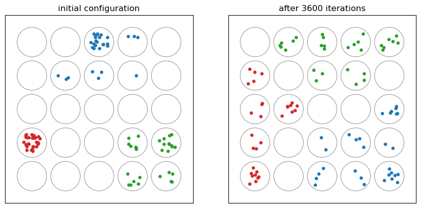
The trained map has separated the three colours into neighbouring regions, and it has done so with a smooth boundary: adjacent cells hold similar observations. That is the property K-means does not have - its labels carry no adjacency, so the same 25 centroids could be permuted at random and mean the same thing.
What the map does not show is density or size. The red cluster is much tighter than the other two, and nothing in the display says so, because the distances used for the layout are map distances. The book makes the same remark about Figure 14.16.
5. The grid in feature space¶
Drawing the prototypes and the lattice edges in shows what “bending the plane” means geometrically. Where the surface has to double back to reach the tight red cluster, edges lie on top of each other - the fold of Figure 14.17.
fig = plt.figure(figsize=(6, 5.5))
ax = fig.add_subplot(111, projection="3d")
for i in range(q1):
    for j in range(q2):
        k = i * q2 + j
        if i + 1 < q1:
            ax.plot(*zip(M[k], M[k + q2]), color="0.4", lw=1)
        if j + 1 < q2:
            ax.plot(*zip(M[k], M[k + 1]), color="0.4", lw=1)
ax.scatter(X[:, 0], X[:, 1], X[:, 2], c=colours, s=10)
ax.scatter(M[:, 0], M[:, 1], M[:, 2], s=70, facecolors="none",
           edgecolors="purple", linewidths=1.4)
ax.set_title("the fitted lattice in feature space")
plt.show()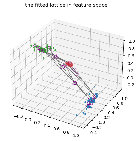
6. The reconstruction error along the way¶
The curve that justifies the constraint is the reconstruction error against the iteration number, with the K-means value as a horizontal line (Figure 14.18).
fig, ax = plt.subplots(figsize=(6.5, 4))
ax.plot(np.arange(1, len(errors) + 1) * len(X), errors, "o-", ms=3, label="SOM")
ax.axhline(km.inertia_, color="tab:red", linestyle="--", label="K-means, 25 centroids")
ax.set_xlabel("iteration (one per observation)")
ax.set_ylabel("reconstruction error")
ax.legend()
ax.set_title("error of the constrained and the unconstrained fit")
plt.show()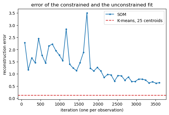
The error falls quickly while the neighbourhood is wide - the map is being unfolded - and approaches the K-means level without reaching it. Reading the last part of the curve is the honest way to answer “is a two-dimensional map appropriate for this data?”, and it is a question about the data, not about the algorithm.
7. The batch version, and the relation to K-means¶
Recomputing the prototype as the weighted mean of the observations that mapped to its neighbours gives the batch SOM:
where the sum runs over observations whose nearest prototype is a map-neighbour of , and is 1 for a rectangular neighbourhood or falls off with the map distance. Two special cases are worth knowing:
a rectangular neighbourhood of radius 0 makes the update “replace each prototype by the mean of its own observations”, which is K-means;
a smooth and a shrinking radius make the batch SOM a discrete version of principal curves, the topic that follows this section in the book.
Between the online and batch versions the trade-off is the familiar one: online adapts to a stream and depends on the schedule, batch is deterministic given the assignment, converges faster, and is what most implementations use by default.
8. Where this is used¶
The closing example of the section is WEBSOM: 12 088 articles from
comp.ai.neural-nets, each turned into a sparse vector of relative term frequencies
over a dictionary of tens of thousands of words (or word pairs), optionally reduced by
a randomised SVD, and then mapped onto a grid whose cells are labelled automatically
from their contents. The map is a browsable index - zooming into a cell shows the
articles - and that is the application the method was built for: not partitioning for
its own sake, but arranging a large collection so that similar things are near each
other on a page.
Summary¶
A SOM is a grid of prototypes with map coordinates; the update moves the winning prototype and its map-neighbours towards the observation (14.46).
The learning rate and the neighbourhood radius both decay; the schedule is part of the definition, which is why the method has no criterion to optimise.
With a single-cell neighbourhood the algorithm is online K-means; the batch form (14.48) with radius 0 is K-means exactly.
The extra error over K-means measures the price of the two-dimensional constraint, and reading it is how you decide whether the map is appropriate.
The output is a display in which neighbouring cells are similar - the property that makes the method useful for browsing large collections.
Exercises¶
Train with from the start. Compare the error curve and the map with K-means labels reshaped onto the grid. What has been lost?
Replace the hard neighbourhood of (14.46) by the Gaussian of (14.47) and compare the final reconstruction errors.
Vary the grid size (, , ) at fixed data. How does the error approach the K-means line, and what does the map look like at ?
Use a hexagonal grid (six neighbours per cell instead of four). Does the display look better, and is the error different?
Run the SOM on 100-dimensional data (e.g. the digits) and measure how much worse the constrained solution is. Is a two-dimensional map still defensible?
Implement the batch version (14.48) with radius 1 and compare the number of iterations needed to reach the same error as the online version.
Sources¶
The definition, (14.46)-(14.48), the half-sphere example with Figures 14.15-14.18, and the WEBSOM application: §14.4 of Hastie et al. (2009), pp. 528-533.
The relation to K-means is the same one used on Clustering-Part2; the online-versus-batch trade-off is the one discussed in Perceptron
-and -Online -Learning. Kohonen’s own account of the method, and the WEBSOM papers, are the references given in the section.
- Hastie, T., Tibshirani, R., & Friedman, J. (2009). The Elements of Statistical Learning: Data Mining, Inference, and Prediction (2nd ed.). Springer. 10.1007/978-0-387-84858-7