Hierarchical Clustering

Where this page sits¶
Section 14.3.12 of Hastie et al. (2009) (pp. 520-528) is the alternative to choosing before you look at the data. Instead of one partition, it builds a nested family of partitions, one per level, and leaves the choice of level to the user - after the structure has been seen.
This page develops the section as it stands: the two paradigms, the dendrogram and what can be read from it, the three linkage rules and the defects of each, the divisive algorithm, and the warnings. An application to colour histograms of images is on the image-clustering page; this page is the method behind it.
What you should be able to do at the end¶
describe agglomerative and divisive clustering and say what each needs from the user;
read a dendrogram, cut it, and know what the height means;
say what a linkage rule is, write the three standard ones, and name the defect of each;
explain why single and complete linkage ignore monotone transformations of the distances while group average does not;
compute the cophenetic correlation and say why it is a weak guarantee.
1. Two paradigms¶
Agglomerative (bottom-up) starts with singleton clusters and, at each of the steps, merges the two clusters with the smallest intergroup dissimilarity. Divisive (top-down) starts with one cluster containing everything and, at each step, splits one existing cluster into two, choosing the split with the largest between-group dissimilarity. Both produce levels and both can be drawn as a rooted binary tree: the leaves are the observations, each internal node is a merge (or a split), and the root is the whole data set.
The tree becomes a picture when the heights are chosen sensibly. All agglomerative methods, and some divisive ones, are monotone: the dissimilarity at which clusters are merged increases with the level. Then the vertical position of a node can be drawn proportional to its merger value, leaves at zero, and the result is a dendrogram.
What the dendrogram is not is a model of the data. The book devotes a paragraph to the caution (p. 522):
Hierarchical methods impose hierarchical structure whether or not such structure actually exists in the data.
Marginal advice follows: the picture is a description of the clustering the algorithm produced, not of the data itself.
2. What the dendrogram can be trusted for¶
Cutting the dendrogram horizontally splits the data into the clusters whose branches cross the cut, which is exactly “stop merging when the dissimilarity exceeds a threshold”. A cut gives a partition; all cuts together give the nested family.
Two numbers measure how well the tree represents the dissimilarities it was built from:
the cophenetic dissimilarity of two observations is the height at which they first join the same cluster;
the cophenetic correlation is the correlation between the input dissimilarities and their cophenetic counterparts.
A high correlation sounds like validation, and the book explains why it is not. The have only distinct values among pairs, so the tree has far fewer degrees of freedom than the matrix; and they must satisfy the ultrametric inequality
for every triple. In a Euclidean picture that forces every triangle to be isosceles with the unequal side no longer than the two equal ones - a very special geometry. General dissimilarities are not like that, so the correlation measures how close the tree comes to a shape it is required to have anyway.
3. Linkage: what “distance between two clusters” means¶
Agglomerative merging needs a dissimilarity between groups, computed from the pairwise dissimilarities between their members. Three rules are standard, with and two groups:
| rule | definition | tendency |
|---|---|---|
| single (SL) | (14.41) | chaining: long thin clusters |
| complete (CL) | (14.42) | compact clusters, may violate closeness |
| group average (GA) | (14.43) | compromise, scale dependent |
Each has a characteristic failure, and the failures are dual:
Single linkage needs only one small dissimilarity for two groups to be called close, so it happily chains observations through close intermediates. The result is a cluster with a huge diameter (14.44), long and thin. This is the classic “chaining” defect.
Complete linkage needs all cross-pairs to be small, so it produces compact clusters - and can put an observation in a cluster whose other members are further from it than members of another cluster are. Compact, but not “close”.
Group average sits between them, and pays for it in scale invariance: applying a monotone increasing transformation to the dissimilarities changes the average, so the result can change. Single and complete use only the ordering of the distances and are invariant under any such . The book uses this invariance as an argument in their favour.
There is one more argument, of the kind this course cares about. If each cluster is a sample from a density , then estimates
a property of the two densities - it converges as . Single linkage converges to zero and complete linkage to infinity regardless of the densities, so it is unclear what population quantity either estimates.
4. The three trees on one data set¶
The data below are three groups in the plane plus a bridge of points joining the first two, which is the configuration single linkage was made to fail on.
import numpy as np
import matplotlib.pyplot as plt
from scipy.cluster.hierarchy import linkage, dendrogram, fcluster, cophenet
from scipy.spatial.distance import pdist, squareform

rng = np.random.default_rng(0)
g1 = rng.normal((-4.0, 0.0), 0.6, size=(8, 2))
g2 = rng.normal((4.0, 0.0), 0.6, size=(8, 2))
g3 = rng.normal((0.0, 5.0), 0.6, size=(8, 2))
bridge = np.column_stack([np.linspace(-3.4, 3.4, 9), np.linspace(-0.4, 0.4, 9)])
X = np.vstack([g1, g2, g3, bridge])
truth = np.r_[np.repeat([0, 1, 2], 8), np.full(9, 3)]
n = len(X)

D1 = pdist(X)
Dfull = squareform(D1)

methods = ["single", "complete", "average"]
fig, axes = plt.subplots(1, 3, figsize=(12, 3.6))
for ax, method in zip(axes, methods):
    Z = linkage(D1, method=method)
    dendrogram(Z, ax=ax, no_labels=True, color_threshold=0)
    c, coph = cophenet(Z, D1)
    ax.set_title(f"{method} linkage\ncophenetic correlation {c:.3f}")
    ax.set_xlabel("observations")
plt.tight_layout()
plt.show()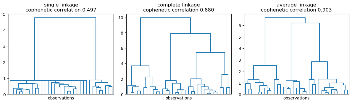
The cophenetic correlation differs across the three panels, and the book’s point is that it does not settle anything: all three trees are valid descriptions of their own merge sequence. What differs is the shape of the answer, and that is visible without any coefficient.
The next cell makes the difference numerical: cut each tree at three clusters and measure the diameter of the widest cluster, and the agreement with the true groups.
from sklearn.metrics import adjusted_rand_score


def diameters(labels, Dfull):
    out = []
    for k in np.unique(labels):
        idx = np.where(labels == k)[0]
        out.append(Dfull[np.ix_(idx, idx)].max() if len(idx) > 1 else 0.0)
    return np.array(out)


print(f"{'method':>9} {'ARI vs truth':>13} {'max diameter':>14} {'clusters':>9}")
for method in methods:
    Z = linkage(D1, method=method)
    labels = fcluster(Z, t=3, criterion="maxclust")
    print(f"{method:>9} {adjusted_rand_score(truth, labels):13.3f} "
          f"{diameters(labels, Dfull).max():14.2f} {len(np.unique(labels)):9d}")
method ARI vs truth max diameter clusters
single 0.271 9.94 3
complete 0.581 5.39 3
average 0.570 4.55 3
Single linkage puts the bridge and both groups it joins into one cluster with a diameter of the order of the whole bridge; complete and average keep the groups compact. On data where the groups are genuinely compact and well separated, all three agree - which is precisely the situation in which the choice does not matter.
5. Scale invariance, checked¶
The claim is that single and complete depend only on the ordering of the dissimilarities, while group average uses their values. The cell below applies - strictly increasing, so the ordering is untouched - rebuilds the three trees from the transformed distances, and compares the resulting three-cluster partitions with the untransformed ones.
D2 = D1 ** 3
print(f"{'method':>9} {'same partition after d -> d^3':>32} {'ARI':>6}")
for method in methods:
    labels_1 = fcluster(linkage(D1, method=method), t=3, criterion="maxclust")
    labels_2 = fcluster(linkage(D2, method=method), t=3, criterion="maxclust")
    same = np.array_equal(labels_1, labels_2)
    print(f"{method:>9} {str(same):>32} {adjusted_rand_score(labels_1, labels_2):6.3f}")
method same partition after d -> d^3 ARI
single True 1.000
complete True 1.000
average False 0.897
Single and complete answer “True”: with the same data and the same ordering, they rebuild exactly the same tree, because and of a monotone function are the monotone function of the and . Group average can answer “False”, and when it does, the reason is that the average of cubes is not the cube of the average: three small distances and one large one trade places.
This is not a curiosity. Distances are often rescaled - to a correlation, to a similarity, to a rank - and the question “does the clustering survive the rescaling?” has a definite answer for two of the three rules and not for the third.
6. Divisive clustering¶
Top-down clustering has been studied far less. Using K-means with at every node is the obvious version, and it inherits the two problems of that method: it depends on a starting configuration, and the sequence of splits need not be monotone, so it cannot be drawn as a proper dendrogram.
The book gives Macnaughton Smith’s algorithm, which avoids both. Start with one group containing everything. Take the observation whose average dissimilarity from the others is largest, and make it the first member of a second group . Then repeatedly move to the observation of for which
is largest, stopping when that difference turns negative. The result is a split into two groups; apply it recursively, choosing at each level the cluster with the largest diameter (14.44) to split next.
def average_to(group, i, Dfull):
    others = [j for j in group if j != i]
    return Dfull[i, others].mean() if others else 0.0


def ms_split(members, Dfull):
    """Macnaughton Smith's two-way split of one group."""
    members = list(members)
    if len(members) < 2:
        return members, []
    first = max(members, key=lambda i: average_to(members, i, Dfull))
    G, H = [i for i in members if i != first], [first]
    while len(G) > 1:
        scores = {i: Dfull[i, H].mean() - average_to(G, i, Dfull) for i in G}
        best = max(scores, key=scores.get)
        if scores[best] <= 0:
            break
        G.remove(best)
        H.append(best)
    return G, H


def divisive(K, Dfull, n):
    groups = [list(range(n))]
    while len(groups) < K:
        groups.sort(key=lambda g: -Dfull[np.ix_(g, g)].max())
        biggest = groups.pop(0)
        A, B = ms_split(biggest, Dfull)
        groups.extend([g for g in (A, B) if g])
    labels = np.zeros(n, dtype=int)
    for k, g in enumerate(groups):
        labels[g] = k
    return labels


for K in (2, 3):
    labels = divisive(K, Dfull, n)
    sizes = sorted(np.bincount(labels), reverse=True)
    print(f"K = {K}: cluster sizes {sizes}, ARI with the true groups "
          f"{adjusted_rand_score(truth, labels):.3f}")
K = 2: cluster sizes [17, 16], ARI with the true groups -0.048
K = 3: cluster sizes [16, 9, 8], ARI with the true groups -0.071
The split sequence is nested by construction - level refines level - which is exactly what K-means cannot promise, and what makes the tumour example prefer a hierarchical answer.
The ARI printed above is the second warning of the section in practice: on this data the first split runs across the groups, so nesting guarantees that the levels refine each other and says nothing about whether any level is right. A hierarchy is a structure the procedure always produces; a useful hierarchy is a property of the data.
7. Ordering the observations¶
Because the leaves of a dendrogram can be flipped at every internal node, the tree fixes a partial order at best. The book adds a rule (S-PLUS’s default: at each merge, put the tighter subtree to the left) and uses it to order both axes of the expression matrix, producing Figure 14.14. The ordering turns a table into a picture: neighbouring columns are similar samples, neighbouring rows are genes that behave alike, and blocks become visible.
Summary¶
Agglomerative clustering merges the closest pair 199 times; divisive clustering splits the most heterogeneous group. Both give a nested family, not one partition.
The dendrogram is readable because merger heights are monotone; the horizontal cut chooses after the fact.
Single linkage chains, complete linkage gives compact but not necessarily close clusters, group average is the compromise that depends on the scale of the distances.
The cophenetic correlation measures how tree-like the dissimilarities are, and the ultrametric inequality says how restrictive “tree-like” is.
K-means with different does not give a nested family; hierarchical clustering does, and that is why the book prefers it for the microarray data.
Exercises¶
Cut each of the three trees at four clusters and recompute the table of ARI and diameters. Which method is stable under the change of ?
Remove the bridge from the data and rerun the comparison. Does single linkage still fail?
Verify the ultrametric inequality for a small tree by computing all cophenetic distances with
cophenet. Find a triple where the inequality is tight.Build a data set where group average changes its partition under , and explain which average moved.
Implement the divisive algorithm with K-means () instead of Macnaughton Smith and check monotonicity of the split heights. Does it ever decrease?
Cluster the iris data with the three linkages, cut at three clusters, and compare with the species labels. Which rule finds setosa first?
Sources¶
The two paradigms, the dendrogram, the cophenetic correlation, (14.40)-(14.45), the Macnaughton Smith algorithm and Figure 14.14: §14.3.12 of Hastie et al. (2009), pp. 520-528.
The application to image histograms, which reuses the same
scipyfunctions: Image-Clustering -Hierarchical. The superiority of a nested family for the tumour data: Tumor
-Microarray -Example, §14.3.8.
- Hastie, T., Tibshirani, R., & Friedman, J. (2009). The Elements of Statistical Learning: Data Mining, Inference, and Prediction (2nd ed.). Springer. 10.1007/978-0-387-84858-7