Vector Quantization and Image Compression

Computer Science Dept, Ferdowsi University of Mashhad
Where this page sits¶
Section 14.3.9 of Hastie et al. (2009) uses K-means for something that has nothing to do with clustering as a descriptive tool: compressing an image. The idea is old and has its own name — vector quantization, VQ — and it is the reason the supervised method of the previous chapter is called Learning Vector Quantization. The two lessons are kept apart, because this one has no labels at all and is measured in bits and decibels instead of error rates.
What you should be able to do at the end¶
describe the encoder and the decoder of a VQ codec, and say what a codeword and a codebook are;
compute the rate of a VQ scheme from the block size and the codebook size, and the distortion from the reconstruction error;
explain why the same K-means code can be a clustering method or a compressor, depending only on what the vectors are;
read a rate/distortion curve and say what the extra bits buy.
1. The idea¶
Cut the image into small blocks. Treat each block as a point in
R^(bs*bs) — a 2×2 block is a point in R^4. Run K-means on the collection of
all blocks of the image. Then:
encoding: store, for every block, the index of its closest centre;
decoding: rebuild the image by replacing every block with that centre.
The centres are called codewords, their set is the codebook, and the
whole thing is lossy: the rebuilt image is not the original. The book’s example
is a 1024×1024 photograph (8 bits per pixel, 1 MB); with K = 200 codewords it
needs 0.239 of the storage, and with K = 4 only 0.0625 of it.
With bs x bs blocks and K codewords, each block costs log2(K) bits, so
and the distortion is the mean squared error between the original and the
rebuilt image. The book reports D = 0.89 at K = 200 and D = 16.95 at
K = 4 (gray levels on the 0–255 scale).
Source
import numpy as np
import matplotlib.pyplot as plt
from sklearn.cluster import KMeans
from skimage import data
from skimage.util import view_as_blocks

%matplotlib inline
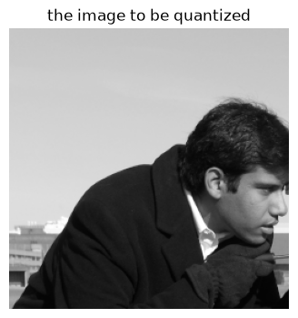
A 256×256 grayscale test image, 8 bits per pixel, is enough to reproduce the
experiment: the arithmetic of the rate does not depend on the picture, and the
smaller image keeps the notebook fast. (The book uses a 1024×1024 portrait; the
same code runs on it and takes K = 200 codewords for 1.91 bits per pixel.)
Source
img = data.camera()[:256, :256]      # 256 x 256, gray levels 0..255
print("shape:", img.shape, "| dtype:", img.dtype, "| range:", img.min(), "-", img.max())

plt.figure(figsize=(4, 4))
plt.imshow(img, cmap="gray", vmin=0, vmax=255)
plt.title("the image to be quantized")
plt.axis("off");
shape: (256, 256) | dtype: uint8 | range: 3 - 255
2. Blocks become vectors¶
view_as_blocks cuts the image without copying overlapping pixels; reshaping the
result gives one row per block. Note what has been gained: the picture is now a
cloud of points in R^4, and K-means does not know — or care — that they came
from an image.
Source
def blocks_of(img, bs):
    """Cut the image into bs x bs blocks; every block becomes a row vector."""
    h, w = img.shape
    grid = view_as_blocks(img, (bs, bs))            # (h/bs, w/bs, bs, bs)
    return grid.reshape(-1, bs * bs).astype(float)


blocks = blocks_of(img, 2)
print("pixels:", img.size, "| blocks:", blocks.shape[0], "| vector length:", blocks.shape[1])
blocks[:3]
pixels: 65536 | blocks: 16384 | vector length: 4
array([[200., 200., 200., 199.],
       [200., 200., 199., 200.],
       [199., 200., 199., 200.]])
3. Encoding and decoding in one function¶
KMeans.fit is the encoder: it builds the codebook and returns the index of
the nearest codeword for every block (labels_). Indexing the codebook with
those labels and folding the vectors back into blocks is the decoder.
Source
def vq_round_trip(img, bs, K, n_init=3, seed=0):
    """Encode with K-means on blocks, then decode; return the rebuilt image and its cost."""
    blocks = blocks_of(img, bs)
    km = KMeans(n_clusters=K, n_init=n_init, max_iter=100, random_state=seed).fit(blocks)

    rec_blocks = km.cluster_centers_[km.labels_]          # decoding
    h, w = img.shape
    rec = rec_blocks.reshape(h // bs, w // bs, bs, bs).transpose(0, 2, 1, 3).reshape(h, w)

    rate = np.log2(K) / (bs * bs)                         # bits per pixel, fixed-length code
    mse = ((img - rec) ** 2).mean()
    return dict(rec=rec, rate=rate, mse=mse,
                psnr=10 * np.log10(255 ** 2 / mse), labels=km.labels_)


print(vq_round_trip(img, 2, 16)["rate"], "bits per pixel for 2x2 blocks, K=16")
1.0 bits per pixel for 2x2 blocks, K=16
4. The rate/distortion table¶
Each row is one codec: a block size (2 x 2 everywhere here) and a codebook size.
K grows geometrically, the rate grows logarithmically — that is the whole
economy of the method.
Source
results = {}
print(f"{'K':>5}{'bits/block':>12}{'rate (bpp)':>12}{'storage':>9}{'MSE':>8}{'PSNR dB':>9}")
for K in (2, 4, 16, 64, 200):
    r = vq_round_trip(img, 2, K)
    results[K] = r
    print(f"{K:>5}{np.log2(K):>12.0f}{r['rate']:>12.2f}{r['rate'] / 8:>9.3f}"
          f"{r['mse']:>8.2f}{r['psnr']:>9.2f}")
K bits/block rate (bpp) storage MSE PSNR dB
2 1 0.25 0.031 489.17 21.24
4 2 0.50 0.062 169.17 25.85
16 4 1.00 0.125 49.73 31.16
64 6 1.50 0.188 19.36 35.26
200 8 1.91 0.239 8.53 38.82
Source
fig, axes = plt.subplots(2, 3, figsize=(11, 7))
axes[0, 0].imshow(img, cmap="gray", vmin=0, vmax=255)
axes[0, 0].set_title("original (8 bpp)")
for ax, K in zip(axes.ravel()[1:], (2, 4, 16, 64, 200)):
    ax.imshow(results[K]["rec"], cmap="gray", vmin=0, vmax=255)
    ax.set_title(f"K = {K},  {results[K]['rate']:.2f} bpp")
for ax in axes.ravel():
    ax.axis("off")
plt.tight_layout();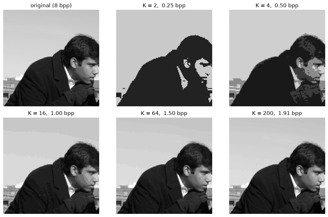
At 0.50 bits per pixel — one sixteenth of the original — the picture is
already recognisable, which is the point of the method. At 0.06 bits per pixel
the blocks win, and the image is a mosaic of 2×2 tiles: sixteen times fewer
codewords than tiles means that neighbouring tiles are forced to share a value.
The same information, plotted as a curve, is the object that compression engineers compare codecs with.
Source
fig, ax = plt.subplots(figsize=(6, 4))
ax.loglog([results[K]["rate"] for K in results], [results[K]["mse"] for K in results], "o-")
for K in results:
    ax.annotate(f"K={K}", (results[K]["rate"], results[K]["mse"]),
                textcoords="offset points", xytext=(6, 4), fontsize=8)
ax.set_xlabel("rate (bits per pixel)")
ax.set_ylabel("distortion (MSE)")
ax.set_title("rate/distortion curve")
ax.grid(alpha=0.3, which="both");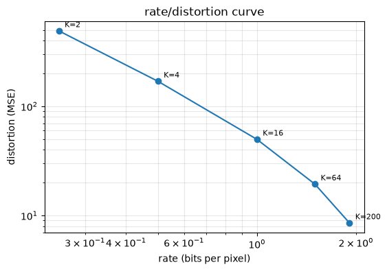
5. Fixed-length or entropy coding?¶
log2(K) bits per block assumes every codeword is equally likely. It is not:
several codewords (plain white, a few grays) are used by thousands of blocks while
others appear a handful of times. Coding the indices with a length proportional
to -log2(p) instead — Shannon’s construction — gives the entropy rate
which is always below the fixed-length rate. The book reports 1.42 and 0.39 bits per pixel for the same two codebooks, against 1.91 and 0.50.
Source
def entropy_rate(labels, bs):
    p = np.bincount(labels) / len(labels)
    p = p[p > 0]
    return -(p * np.log2(p)).sum() / (bs * bs)


print(f"{'K':>5}{'fixed-length':>15}{'entropy code':>15}")
for K, r in results.items():
    print(f"{K:>5}{r['rate']:>15.2f}{entropy_rate(r['labels'], 2):>15.2f}")
K fixed-length entropy code
2 0.25 0.25
4 0.50 0.40
16 1.00 0.82
64 1.50 1.11
200 1.91 1.45
6. The other knob: block size¶
The rate formula has bs in the denominator twice over, so large blocks are
cheap per pixel — and expensive in fidelity, because a block is forced to become
one of K average patches. With the codebook held at K = 16 and the block size
doubling, the rate falls by a factor of four each time:
Source
fig, axes = plt.subplots(1, 3, figsize=(11, 4))
for ax, bs in zip(axes, (2, 4, 8)):
    r = vq_round_trip(img, bs, 16)
    ax.imshow(r["rec"], cmap="gray", vmin=0, vmax=255)
    ax.set_title(f"{bs}x{bs} blocks, K=16\n{r['rate']:.3f} bpp, MSE={r['mse']:.1f}")
    ax.axis("off")
plt.tight_layout();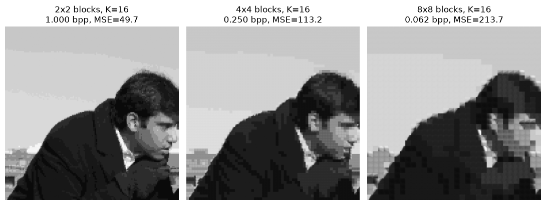
The 8×8 version is cheapest and worst: the tiles are visible as squares, and edges of objects become staircases. Real codecs therefore use larger codebooks with small blocks, or transform the block before quantizing (the JPEG family), which is the same trade-off expressed in a different basis.
Summary¶
Vector quantization replaces each block by the index of the nearest codeword; the set of codewords is the codebook.
The encoder is
KMeans.fit, the decoder iscodebook[labels]; the algorithm is Lloyd’s, and nothing in it knows that the vectors came from an image.The rate is
log2(K)/bs^2bits per pixel, and the distortion is the MSE of the reconstruction; the pair traces a rate/distortion curve.Fixed-length coding wastes bits when the codeword distribution is skewed; entropy coding of the same indices lowers the rate without touching the distortion.
Block size and codebook size are two ways to spend the same bit budget; the visible artifacts (2×2 tiles, staircase edges) tell you which one is being spent.
This is where the name Learning Vector Quantization comes from — but VQ itself uses no labels, and is the subject of a page of its own.
Exercises¶
Reproduce the book’s setting: take a 1024×1024 image, 2×2 blocks,
K = 200, and check the storage fraction0.239. Where does the remaining difference from the ideal come from?Compute the variable-length rate of a codebook built on 4×4 blocks and compare it with the fixed-length rate. Which codewords dominate?
Replace K-means by a random codebook (sample
Kblocks and use them as centres). How much worse is the distortion at the same rate, and why?Quantize the color image: blocks of shape
(2, 2, 3), vectors inR^12. Compare rate and visual quality with the gray version.Plot distortion against rate for
bs = 2, 4andK = 2..256on one axes. Is one block size uniformly better, or do the curves cross?What would a lossless version of block clustering look like? (Hint: the book reports that entropy coding the original image reaches 4.48 bits per pixel, so lossless block coding can aim for that.)
Sources¶
The method, the worked example and the reported numbers (1.91 and 0.50 bits per pixel,
D = 0.89and16.95, entropy rates 1.42 and 0.39): §14.3.9 of Hastie et al. (2009), pp. 514–516. Figures here are produced by the code above on a different test image, so the distortions are not directly comparable with the book’s.Gersho and Gray, Vector Quantization and Signal Compression, is the reference the book cites for the method itself.
The supervised variant of the same idea — where the prototypes carry class labels — is Learning Vector Quantization.
- Hastie, T., Tibshirani, R., & Friedman, J. (2009). The Elements of Statistical Learning: Data Mining, Inference, and Prediction (2nd ed.). Springer. 10.1007/978-0-387-84858-7