SVD for Image Compression¶

Mahmood Amintoosi, Fall 2026

Computer Science Dept, Ferdowsi University of Mashhad

Jupyter is an interactive browser based notebook environment where we can combine text, code execution and visualization. It supports multiple programming languages through it’s language specific kernel plugins. However, it is widely used with Python in scientific computing and data science communities. The availability of large number of high quality open source libraries useful for many tasks in scientific computing,numerical linear algebra, machine learning and visualization ensures that Python is being widely used in these fields. Jupyter notebooks are an excellent environment for learning and teaching because of the interactivity.

In this short blogpost, I will explore few topics to illustrate the interactivity of the jupyter environment and the availability of high quality libraries in the python ecosystem.

• Montecarlo calculation of $\pi$

• Image Compression using Singular value decomposition

A note on installation of jupyter¶

Installation of jupyter and other important packages individually is cumbersome. Thanks to Anaconda we have Anaconda python distribution in which almost all of the useful packages are bundled. Install anaconda.

But it is even better not setting up any python environment at all on your computer. Instead, you can use free online python environments- colab notebooks from google or sagemaker studio lab notebook from aws. Watch this video from the twitter user 1littlecoder on getting started with sagemaker studio lab.

Montecarlo calculation of $\pi$¶

I had earlier written about calculating the mathematical constant $\pi$ using montecarlo method. It involves generating random points on a unit square and counting the number of points inside the unit quarter circle. We will write a function mc_pi to calculate $\pi$. In that function, we will also visualize the process of montecarlo simulation using matplotlib library.

We are able to write the function mc_pi without making use of any explicit for loops - thanks to vectorization features in numpy library. Due to a concept called broadcasting in numpy, we are able to subtract a vector from a scalar (1.0 - unit_circle_x**2 ) to compute the y co-ordinate of the unit circle.

Now we will make use of ipywidgets module to pass the parameter interactively to the function mc_pi. ipywidgets module provide widgets to generate the UI controls in the notebook itself with which the user can interact. We can drag the slider and observe how the value of pi calculated by mc_pi function changes with the number of trials.

SVD and Image compression¶

Now we will explore how to apply Singular Value Decomposition of a matrix to the problem of image compression. SVD decomposes a rectangular matrix $M$ to a three parts. $M=U\Sigma V^T$ -

• $U$ - matrix of left singular vectors in the columns

• $\Sigma$ - diagonal matrix with singular values

• $V$ - matrix of right singular vectors in the columns

SVD in effect involves reconstructing the original matrix as a linear combination of several rank one matrices. A rank one matrix can be expressed as a outer product of two column vectors.

$M=\sigma_1u_1v_1^T+\sigma_2u_2v_2^T+\sigma_3u_3v_3^T+\sigma_3u_3v_3^T+....$ . A matrix of rank r will have r terms of these.

Here $\sigma_1,\sigma_2,\sigma_3 ...$ are singular values. $u_1,u_2,u_3 ...$ and $v_1,v_2,v_3 ...$ are left and right singular vectors respectively.

Image compression using SVD involves taking advantage of the fact that very few of the singular values are large. Although images from the real world are of full rank, they have low effective rank which means that only few of the singular values of the SVD of images will be large.

skimage image processing library¶

We will use skimage image processing library (from sci-kit family of packages) for working with images in python. skimage has a module called data which makes available a set of images for exploration. We will load some images and convert them into a gray scale format. These images are stored in a python dict object gray_images.

svd in python¶

We will use numpy.linalg library’s svd function to compute svd of a matrix in python. The svd function returns U,s,V .

• U has left singular vectors in the columns

• s is rank 1 numpy array with singular values

• V has right singular vectors in the rows -equivalent to $V^T$ in traditional linear algebra literature

The reconstructed approximation of the original matrix is done using a subset of singular vectors as below in the compress_svd function . We use numpy array slicing to select k singular vectors and values. Instead of storing $m\times n$ values for the original image, we can now store $k(m+n)+k$ values

       reconst_matrix = np.dot(U[:,:k],np.dot(np.diag(s[:k]),V[:k,:]))

Compress gray scale images¶

The function compress_show_gray_images below takes in the image name (img_name) and number of singular values/vectors(k) to be used in the compressed reconstruction. It also plots the singular values and the image.

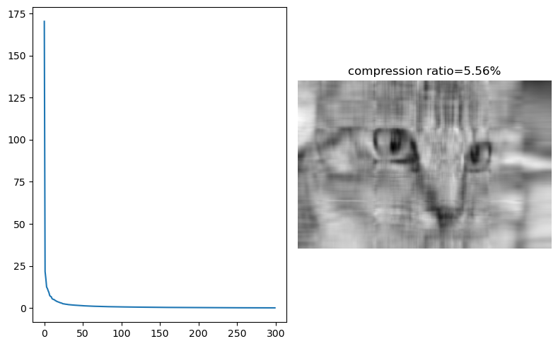
Use the below interactive widget to explore how the quality of the reconstructed image varies with $k$

Load color images¶

Compress color images¶

Color images are represented in python as 3 dimensional numpy arrays - the third dimension to represent the color values (red,green blue). However, svd method is applicable to two dimensional matrices. So we have to find a way to convert the 3 dimensional array to 2 dimensional arrays, apply svd and reconstruct it back as a 3 dimensional array . There are two ways to do it. We will show both these methods below .

• reshape method

• Layer method

Reshape method to compress a color image¶

This method involves flattening the third dimension of the image array into the second dimension using numpy’s reshape method .

image_reshaped = image.reshape((original_shape[0],original_shape[1]*3))

The svd decomposition is applied on the resulting reshaped array and reconstructed with the desired number of singular values/vectors. The image array is reshaped back to the three dimensions by another call to reshape method.

image_reconst = image_reconst.reshape(original_shape)

Here is the interactive widget to explore image compression of color images using the reshape method. By dragging the slider to vary $k$, observe how image quality varies. Also, we can explore different images by selecting through the drop down widget.

Layers method to compress color images¶

In the function compress_show_color_images_layer, we treat a color image as a stack of 3 seperate two dimensional images (Red,blue and green layers) . We apply the truncated svd reconstruction on each two dimensional layer seperately.

image_reconst_layers = [compress_svd(image[:,:,i],k)[0] for i in range(3)]

And we put back the reconstructed layers together.

image_reconst = np.zeros(image.shape)
for i in range(3):
   image_reconst[:,:,i] = image_reconst_layers[i]

Here is the widget to explore layers method of compressing color images.