Principal Component Analysis, Part 2
From mathematical foundations to practical implementation
Principal Component Analysis (PCA) is a fundamental dimensionality reduction technique that identifies an optimal -dimensional subspace capturing the maximum variance in the data. Its mathematical foundation rests on finding orthogonal directions — called principal components — that sequentially maximize the projected variance.
Given a centered data matrix , we seek unit vectors that maximize the variance of projected data :
This optimization leads to the key eigenvalue problem:
where is a covariance matrix.
In the following sections, we will systematically derive the solution to this problem and demonstrate its geometric interpretation.
Source
import numpy as np
import matplotlib.pyplot as plt
from sklearn.decomposition import PCA

# Generate synthetic data with elliptical shape
np.random.seed(42)
n_samples = 100
mean = [0, 0]
cov = [[1, 0.6], [0.6, 0.5]]  # Covariance matrix for elliptical distribution
data = np.random.multivariate_normal(mean, cov, n_samples)

# Center the data
centered_data = data - np.mean(data, axis=0)

# Perform PCA
pca = PCA()
pca.fit(centered_data)
components = pca.components_
explained_variance = pca.explained_variance_ratio_

# Project data onto principal components
projected_data = pca.transform(centered_data)

# Create figure
plt.figure(figsize=(12, 8))

# Plot original data
plt.scatter(centered_data[:, 0], centered_data[:, 1], alpha=0.5, label='Original Data', color='blue')

# Plot principal components as elegant vectors
pc_scale = 2.1  # Scaling factor for PC vectors
plt.quiver(0, 0, components[0,0]*pc_scale, components[0,1]*pc_scale,
          color='lightcoral', scale=1, scale_units='xy', angles='xy', width=0.002,
          label=f'PC1 (Variance: {100*explained_variance[0]:.1f}%)')
plt.quiver(0, 0, components[1,0]*pc_scale, components[1,1]*pc_scale,
          color='lightgreen', scale=1, scale_units='xy', angles='xy', width=0.002,
          label=f'PC2 (Variance: {100*explained_variance[1]:.1f}%)')

# Plot projections onto PC1 (first principal component)
for point in centered_data:
    projection_pc1 = np.dot(point, components[0]) * components[0]
    plt.plot([point[0], projection_pc1[0]], [point[1], projection_pc1[1]],
             'r--', alpha=0.3, linewidth=0.7)

# Plot projections onto PC2 (second principal component)
for point in centered_data:
    projection_pc2 = np.dot(point, components[1]) * components[1]
    plt.plot([point[0], projection_pc2[0]], [point[1], projection_pc2[1]],
             'g--', alpha=0.2, linewidth=0.6)

# Plot the projected points on PC1
projected_pc1 = np.dot(projected_data[:, 0][:, np.newaxis], components[0:1, :])
plt.scatter(projected_pc1[:, 0], projected_pc1[:, 1], color='red', alpha=0.7,
            label='Projections on PC1', s=30)

# Plot the projected points on PC2
projected_pc2 = np.dot(projected_data[:, 1][:, np.newaxis], components[1:2, :])
plt.scatter(projected_pc2[:, 0], projected_pc2[:, 1], color='green', alpha=0.7,
            label='Projections on PC2', s=30)

# Add annotations and legend
plt.axhline(0, color='black', linestyle='--', alpha=0.2)
plt.axvline(0, color='black', linestyle='--', alpha=0.2)
plt.xlabel('Feature 1')
plt.ylabel('Feature 2')
plt.title('PCA: Principal Components and Data Projections\n'
          f'PC1 explains {100*explained_variance[0]:.1f}% of variance\n'
          f'PC2 explains {100*explained_variance[1]:.1f}% of variance')
plt.legend(loc="lower right")
plt.grid(alpha=0.2)
plt.axis('equal')
plt.show()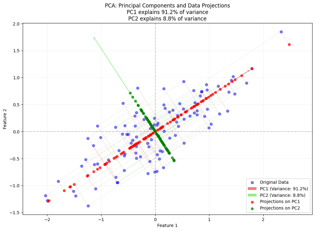
Linear Algebra Foundations
Data Matrix Representation
A data matrix with rows (samples) and columns (features) can be written as:
Each row represents one sample in -dimensional space.
Source
import numpy as np
import matplotlib.pyplot as plt
from sklearn.datasets import load_iris, make_blobs
from sklearn.decomposition import PCA
import seaborn as sns

# Set style for better plots
plt.style.use('seaborn-v0_8')
np.random.seed(42)
Vector Operations
Dot Product
Vector Length (Norm)
Unit Vector
Distance between Vectors
Angle between Vectors
# Example: Vector operations
a = np.array([3, 4])
b = np.array([1, 2])

# Dot product
dot_product = np.dot(a, b)
print(f"Dot product: {dot_product}")

# Vector norms
norm_a = np.linalg.norm(a)
norm_b = np.linalg.norm(b)
print(f"Norm of a: {norm_a:.2f}")
print(f"Norm of b: {norm_b:.2f}")

# Angle between vectors
cos_theta = dot_product / (norm_a * norm_b)
theta_rad = np.arccos(cos_theta)
theta_deg = np.degrees(theta_rad)
print(f"Angle between vectors: {theta_deg:.2f} degrees")
Dot product: 11
Norm of a: 5.00
Norm of b: 2.24
Angle between vectors: 10.30 degrees
Vector Projections (Derivation & Geometric Intuition)
Derivation of Projection Formula
We begin with fundamental vector operations to derive the projection formula naturally:
Dot Product and Angle Relationship:
From our previous definitions, we know:This measures alignment between vectors.
Scalar Projection (Length of Shadow):
The length of 's shadow along is:For unit vectors, this simplifies to .
Vector Projection:
To get the vector form, we multiply the scalar projection by 's unit vector:
Final Projection Formula
Key Insights:
Dot Product Interpretation:
The numerator measures alignment
The denominator normalizes for vector length
Special Case - Unit Vector: When :
Geometric Meaning:
is 's shadow on
The residual is orthogonal to
Example
Let and .
Step 1: Compute .
Step 2: Compute .
Step 3: Projection .
Perpendicular Component: .
Interpretation:
Since points along the x-axis, retains only the x-component of , and captures the remaining y-component, which is orthogonal to .
Connection to PCA:
This projection concept is the geometric heart of PCA. In the next section we extend it to multiple dimensions, leading to the PCA solution via eigenvalue decomposition.
# Example: Vector projection
def project_vector(b, a):
    """Project vector b onto vector a"""
    projection = (np.dot(a, b) / np.dot(a, a)) * a
    perpendicular = b - projection
    return projection, perpendicular

# Example vectors
a = np.array([1, 0])  # Direction vector
b = np.array([3, 2])  # Vector to project

b_parallel, b_perp = project_vector(b, a)

print(f"Original vector b: {b}")
print(f"Projection onto a: {b_parallel}")
print(f"Perpendicular component: {b_perp}")
print(f"Verification (should equal b): {b_parallel + b_perp}")
Original vector b: [3 2]
Projection onto a: [3. 0.]
Perpendicular component: [0. 2.]
Verification (should equal b): [3. 2.]
Source
plt.rcParams['font.family'] = 'DejaVu Sans'

# Visualization of vector projection
plt.figure(figsize=(10, 5))

# Plot vectors
plt.quiver(0, 0, a[0], a[1], angles='xy', scale_units='xy', scale=1, color='red', width=0.005, label='Direction vector a')
plt.quiver(0, 0, b[0], b[1], angles='xy', scale_units='xy', scale=1, color='blue', width=0.003, label='Original vector b')
plt.quiver(0, 0, b_parallel[0], b_parallel[1], angles='xy', scale_units='xy', scale=1, color='green', width=0.003, label='Projection b∥')
plt.quiver(b_parallel[0], b_parallel[1], b_perp[0], b_perp[1], angles='xy', scale_units='xy', scale=1, color='orange', width=0.003, label='Perpendicular b⊥')

# Add dotted line to show projection
plt.plot([b[0], b_parallel[0]], [b[1], b_parallel[1]], 'k--', alpha=0.5)

# Set axis limits with some padding
padding = 0.5
plt.xlim(min(0, b[0], b_parallel[0]) - padding, max(a[0], b[0], b_parallel[0]) + padding)
plt.ylim(min(0, b[1], b_parallel[1]) - padding, max(a[1], b[1], b_parallel[1]) + padding)
# plt.xlim(-0.5, 3.5)
# plt.ylim(-0.5, 2.5)
plt.grid(True, alpha=0.3)
plt.axis('equal')
plt.legend()
plt.title('Vector Projection Demonstration')
plt.xlabel('X')
plt.ylabel('Y')
plt.show()

# Print the vectors and their magnitudes
print(f"Vector a: {a}, magnitude: {np.linalg.norm(a):.2f}")
print(f"Vector b: {b}, magnitude: {np.linalg.norm(b):.2f}")
print(f"b_parallel: {b_parallel}, magnitude: {np.linalg.norm(b_parallel):.2f}")
print(f"b_perpendicular: {b_perp}, magnitude: {np.linalg.norm(b_perp):.2f}")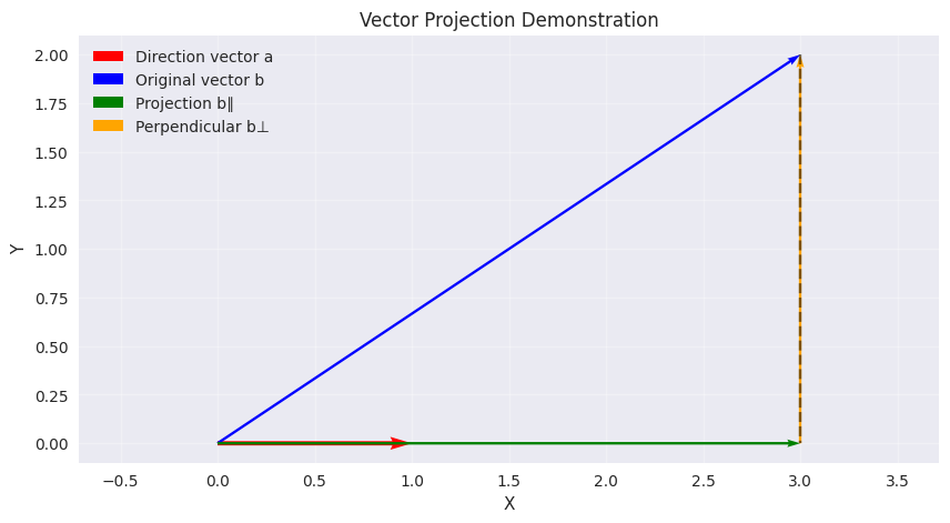
Vector a: [1 0], magnitude: 1.00
Vector b: [3 2], magnitude: 3.61
b_parallel: [3. 0.], magnitude: 3.00
b_perpendicular: [0. 2.], magnitude: 2.00
Basis Transformation
Change of Basis
Any vector can be expressed in terms of a new orthonormal basis :
where has the new basis vectors as its columns, and holds the coordinates of in the new basis:
This works because orthonormality gives , so the coordinate in direction is simply the dot product .
# Example: Basis transformation
# Original vector
x = np.array([0.5, 1, 2])

# Standard basis (i, j, k)
standard_basis = np.eye(3)
i = standard_basis[:, 0]
j = standard_basis[:, 1]
k = standard_basis[:, 2]

print(f"Original vector x: {x}")
print(f"In standard basis: {x[0]}i + {x[1]}j + {x[2]}k")

# Create a new orthonormal basis (rotated 45° in xy-plane)
u1 = np.array([1/np.sqrt(2), 1/np.sqrt(2), 0])
u2 = np.array([-1/np.sqrt(2), 1/np.sqrt(2), 0])
u3 = np.array([0, 0, 1])

# New basis matrix
U = np.column_stack([u1, u2, u3])
print(U)
Original vector x: [0.5 1. 2. ]
In standard basis: 0.5i + 1.0j + 2.0k
[[ 0.70710678 -0.70710678 0. ]
[ 0.70710678 0.70710678 0. ]
[ 0. 0. 1. ]]
Source
# Create 3D plot
fig = plt.figure(figsize=(15, 5))

# Plot 1: Original vector and standard basis
ax1 = fig.add_subplot(121, projection='3d')
ax1.set_title('Original Vector and Standard Basis')

# Plot standard basis vectors
ax1.quiver(0, 0, 0, i[0], i[1], i[2], color='r', label='i')
ax1.quiver(0, 0, 0, j[0], j[1], j[2], color='g', label='j')
ax1.quiver(0, 0, 0, k[0], k[1], k[2], color='b', label='k')

# Plot original vector
ax1.quiver(0, 0, 0, x[0], x[1], x[2], color='purple', label='x')

# Plot xy-plane for reference
xx, yy = np.meshgrid(range(-2, 3), range(-2, 3))
zz = np.zeros_like(xx)
ax1.plot_surface(xx, yy, zz, alpha=0.1, color='gray')

# Plot 2: Rotated basis and transformed vector
ax2 = fig.add_subplot(122, projection='3d')
ax2.set_title('Rotated Basis and Transformed Vector')

# Plot rotated basis vectors
ax2.quiver(0, 0, 0, u1[0], u1[1], u1[2], color='r', label='u1')
ax2.quiver(0, 0, 0, u2[0], u2[1], u2[2], color='g', label='u2')
ax2.quiver(0, 0, 0, u3[0], u3[1], u3[2], color='b', label='u3')

# Plot original vector
ax2.quiver(0, 0, 0, x[0], x[1], x[2], color='purple', label='x')

# Plot rotated xy-plane
R = np.array([[1/np.sqrt(2), -1/np.sqrt(2), 0],
              [1/np.sqrt(2), 1/np.sqrt(2), 0],
              [0, 0, 1]])
rotated_points = R @ np.array([xx.flatten(), yy.flatten(), zz.flatten()])
rotated_xx = rotated_points[0].reshape(xx.shape)
rotated_yy = rotated_points[1].reshape(yy.shape)
rotated_zz = rotated_points[2].reshape(zz.shape)
ax2.plot_surface(rotated_xx, rotated_yy, rotated_zz, alpha=0.1, color='gray')

# Set equal aspects and labels
for ax in [ax1, ax2]:
    ax.set_xlabel('X')
    ax.set_ylabel('Y')
    ax.set_zlabel('Z')
    ax.set_xlim([-2, 2])
    ax.set_ylim([-2, 2])
    ax.set_zlim([-2, 2])
    # ax.set_xticks([])  # Disable x-axis numbers
    ax.set_yticks([])  # Disable y-axis numbers
    ax.set_zticks([])  # Disable z-axis numbers
    ax.legend()

plt.tight_layout()
plt.show()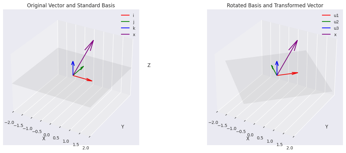
Rotation Matrix Mathematical Foundation
2D Rotation Fundamentals
A rotation matrix transforms vectors by rotating them through a specified angle θ while preserving their length. For a 45° rotation in the xy-plane (θ = π/4 radians), the fundamental rotation matrix is:
For θ = 45°:
Thus, the 45° rotation matrix becomes:
Basis Transformation
In the previous code, this rotation matrix defines new basis vectors:
u1 = np.array([1/np.sqrt(2), 1/np.sqrt(2), 0])  # Rotated x-axis
u2 = np.array([-1/np.sqrt(2), 1/np.sqrt(2), 0]) # Rotated y-axis
u3 = np.array([0, 0, 1])                        # Unchanged z-axis
These form an orthonormal basis:
: Original x-axis rotated 45° counterclockwise
: Original y-axis rotated 45° counterclockwise
: Original z-axis (unchanged)
Key Properties
Orthonormality:
Determinant: (preserves orientation)
Inverse: (transpose reverses rotation)
Vector Transformation
For any vector , the rotated version is:
This matches our basis transformation approach where:
Why This Works
The columns of are exactly the images of the standard basis vectors under the rotation. When we multiply:
So tells us precisely where each axis goes — which is why its columns form the new basis.
# Transform to new basis
a = U.T @ x

print(f"\nIn new basis: {a[0]:.2f}u1 + {a[1]:.2f}u2 + {a[2]:.2f}u3")

# Verify: transform back to original
x_reconstructed = U @ a
print(f"\nReconstructed x: {x_reconstructed}")
print(f"Reconstruction error: {np.linalg.norm(x - x_reconstructed):.10f}")
In new basis: 1.06u1 + 0.35u2 + 2.00u3

Reconstructed x: [0.5 1.  2. ]
Reconstruction error: 0.0000000000
PCA Mathematical Foundation
Variance Maximization Problem
PCA seeks an orthonormal basis that captures maximal variance in the data through sequential optimization:
First Principal Component:
Find unit vector maximizing projected variance:Subsequent Components:
Each is found by maximizing variance orthogonal to previous components:
In short, the first principal component is the direction of greatest spread in the data. Each subsequent component must be orthogonal to all previous ones, ensuring it captures genuinely new, independent information.
Finding the first principal component
We seek a unit vector that maximizes the variance of the projected data:
where is the mean of the projected values (using linearity of the dot product).
Expanding the variance:
Let denote the scalar projection of the -th sample.
The variance becomes:
Let denote the centered data points. Expanding step by step:
Use the identity , noting that :
Rearrange, grouping between and :
Pull and outside the sum:
Recognize the sample covariance matrix :
Equivalently, using the centered data matrix :
Hence the variance of the projected data is:
Constrained Optimization via Lagrange Multipliers
We maximize the projected variance subject to . Introducing Lagrange multiplier , the Lagrangian is:
Solution
Setting the gradient with respect to to zero:
This is precisely the eigenvalue equation: must be an eigenvector of the covariance matrix , with the corresponding eigenvalue.
Choosing the Right Eigenvalue
Substituting back into the variance expression:
The projected variance equals the eigenvalue . To maximize variance we therefore pick , the largest eigenvalue of . The corresponding eigenvector defines the direction of maximum variance — the first principal component.
Source
import numpy as np
import matplotlib.pyplot as plt

# Generate synthetic data
np.random.seed(42)
mean = [0, 0]
cov = [[1, 0.6], [0.6, 0.5]]
X = np.random.multivariate_normal(mean, cov, 100)
# Center the data
X_mean = np.mean(X, axis=0)
Z = X - X_mean
# Compute covariance matrix
cov_matrix = np.dot(Z.T, Z) / (len(Z) - 1)
# Compute eigenvalues and eigenvectors
eigenvalues, eigenvectors = np.linalg.eigh(cov_matrix)
# Sort by descending eigenvalues
idx = eigenvalues.argsort()[::-1]
eigenvalues = eigenvalues[idx]
eigenvectors = eigenvectors[:, idx]
# Extract PC1 (first principal component)
u1 = eigenvectors[:, 0]
λ1 = eigenvalues[0]
print(f"u1 = {u1}, λ1 = {λ1:.2f}")u1 = [-0.83818843 -0.54538075], λ1 = 1.03
Source
# Create figure
plt.figure(figsize=(8, 6))

# Plot original centered data
plt.scatter(Z[:, 0], Z[:, 1], alpha=0.9, label='Original Data (Centered)')

# Plot PC1 direction (scaled by standard deviation)
plt.quiver(0, 0, u1[0]*2*np.sqrt(λ1), u1[1]*2*np.sqrt(λ1),
           color='green', scale=1, scale_units='xy', angles='xy', width=0.007,
           label=f'PC1 (λ={λ1:.2f})')

# Project data onto PC1
projections = np.outer(Z @ u1, u1)  # Projection vectors

# Plot projections
plt.scatter(projections[:, 0], projections[:, 1], color='red', alpha=0.7,
           s=30, label='Projections on PC1')

# Draw projection lines
for point, proj in zip(Z, projections):
    plt.plot([point[0], proj[0]], [point[1], proj[1]],
             'r--', alpha=0.3, linewidth=0.7)

# Formatting
plt.axhline(0, color='black', linestyle='--', alpha=0.2)
plt.axvline(0, color='black', linestyle='--', alpha=0.2)
plt.title('First Principal Component and Projections\n(Maximum Variance Direction)')
plt.xlabel('Feature 1')
plt.ylabel('Feature 2')
plt.legend()
plt.grid(alpha=0.2)
plt.axis('equal')
plt.tight_layout()
plt.show()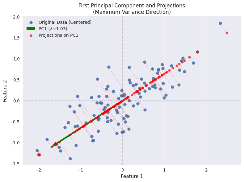
PCA Algorithm
Given a data matrix :
Center the data:
Compute the covariance matrix:
Compute eigenvalues and eigenvectors of
Sort eigenvalues in descending order
Select the top eigenvectors as the principal components
Project the data:
def pca_from_scratch(X, n_components):
    """
    Implement PCA from scratch

    Parameters:
    X: data matrix (n_samples, n_features)
    n_components: number of principal components to keep

    Returns:
    X_transformed: transformed data
    components: principal components
    eigenvalues: eigenvalues
    mean: data mean
    """
    # Step 1: Center the data
    X_mean = np.mean(X, axis=0)
    Z = X - X_mean

    # Step 2: Compute covariance matrix
    n_samples = X.shape[0]
    cov_matrix = np.dot(Z.T, Z) / (n_samples - 1)

    # Step 3: Compute eigenvalues and eigenvectors
    eigenvalues, eigenvectors = np.linalg.eigh(cov_matrix)

    # Step 4: Sort eigenvalues and eigenvectors in descending order
    idx = eigenvalues.argsort()[::-1]
    eigenvalues = eigenvalues[idx]
    eigenvectors = eigenvectors[:, idx]

    # Step 5: Select top n_components
    components = eigenvectors[:, :n_components]

    # Step 6: Project the data
    X_transformed = np.dot(Z, components)

    return X_transformed, components, eigenvalues, X_mean

def reconstruct_data(X_transformed, components, mean):
    """Reconstruct original data from PCA representation"""
    X_reconstructed = np.dot(X_transformed, components.T) + mean
    return X_reconstructed
PCA Workflow: From Single Sample to Full Matrix
Projection & Reconstruction (Single Data Point)
Step 1: Mean-Centering
Given a raw data vector:
Subtract the mean vector:
where is the mean of all samples.
Step 2: Projection (Dimensionality Reduction)
Project onto the first principal components (PCs) : (scalar, projection of onto )
The reduced representation (in PCA space) is:
Step 3: Reconstruction (Approximation)
Reconstruct the centered data using the PCs:
Add back the mean to return to original space:
Geometric Interpretation
The reconstruction is the closest approximation of using only directions.
The error comes from discarding the remaining PCs.
Generalization to Full Data Matrix
Step 1: Mean-Centering (Matrix Form)
Original data matrix:
Mean-centered data:
where is a column vector of ones.
Step 2: Projection (PCA Transformation)
Project all samples onto the first PCs ():
Each row of contains the reduced representation of a sample.
Step 3: Reconstruction (Matrix Form)
Reconstruct the centered data:
= -th column of (scores for PC ).
Each term is a rank-1 matrix.
Return to original space:
Connection to Python Implementation
Projection (Dimensionality Reduction)
X_transformed = Z @ U_r # ≡ Z U_r (n × r matrix)Reconstruction
Z_recon = X_transformed @ U_r.T  # ≡ A U_r^T (n × d)
X_recon = Z_recon + mean        # Add back mean
Key Takeaways
Single Sample Full Matrix:
Start with a single vector to understand projection/reconstruction.
Generalize to the full dataset using matrix operations.
Lossy Compression:
Keeping only PCs means the reconstruction is approximate.
The error depends on the discarded eigenvalues.
PCA as a Rotation:
Projection = Rotate data to align with maximum variance directions.
Reconstruction = Rotate back, using only the most important directions.
Equivalence of PCA’s Two Optimization Perspectives and Error Analysis (Further Reading)
PCA can be derived from two equivalent perspectives:
Variance Maximization: Find directions that maximize projected variance.
Reconstruction Error Minimization: Find directions that minimize the mean squared reconstruction error.
We’ll prove their equivalence mathematically and analyze the error.
1. Variance Maximization Formulation
Goal: Find unit vector that maximizes the variance of projected data:
The solution is the eigenvector of with largest eigenvalue.
2. Reconstruction Error Minimization
Goal: Find that minimizes the MSE between original data and its reconstruction :
3. Proof of Equivalence
Expand the reconstruction error:
Thus, the MSE becomes:
Key Observations:
The term is constant (total variance in data).
Minimizing MSE is equivalent to maximizing (projected variance).
4. Error Analysis in PCA
Projection and Residual Components
For a data point (centered) and its reconstruction using PCs:
Error vector: .
Mean Squared Error (MSE) Derivation
The total MSE across all samples is:
Link to Eigenvalues
By definition, the variance along is:
Thus:
5. Conclusion and Summary
Dual Formulations: Variance maximization and error minimization are equivalent in PCA.
Eigenvalue Interpretation: The MSE equals the sum of discarded eigenvalues because:
Each represents variance along PC .
Discarding PCs to loses exactly variance.
Optimality: PCA’s solution simultaneously maximizes preserved variance and minimizes reconstruction error.
Key Relationships:
| Concept | Formula | Interpretation |
|---|---|---|
| Projection | Reconstruction using top PCs | |
| Error | Residual from discarded PCs | |
| MSE | Sum of variances of discarded PCs |
Source
# Load the Iris dataset
iris = load_iris()
X_iris = iris.data
y_iris = iris.target
feature_names = iris.feature_names

print(f"Original data shape: {X_iris.shape}")
print(f"Features: {feature_names}")

# Apply PCA
X_pca, components, eigenvalues, mean = pca_from_scratch(X_iris, n_components=2)

# Calculate explained variance ratio
total_var = eigenvalues.sum()
explained_var_ratio = eigenvalues[:2] / total_var

print(f"\nExplained variance ratio:")
print(f"PC1: {explained_var_ratio[0]:.3f} ({explained_var_ratio[0]*100:.1f}%)")
print(f"PC2: {explained_var_ratio[1]:.3f} ({explained_var_ratio[1]*100:.1f}%)")
print(f"Total: {explained_var_ratio.sum():.3f} ({explained_var_ratio.sum()*100:.1f}%)")
Original data shape: (150, 4)
Features: ['sepal length (cm)', 'sepal width (cm)', 'petal length (cm)', 'petal width (cm)']
Explained variance ratio:
PC1: 0.925 (92.5%)
PC2: 0.053 (5.3%)
Total: 0.978 (97.8%)
Source
# Visualize the results
plt.figure(figsize=(15, 5))

# Plot 1: Original data (first two features)
plt.subplot(1, 3, 1)
scatter = plt.scatter(X_iris[:, 0], X_iris[:, 1], c=y_iris, cmap='viridis')
plt.xlabel(feature_names[0])
plt.ylabel(feature_names[1])
plt.title('Original Data (First 2 Features)')
plt.colorbar(scatter)

# Plot 2: PCA transformed data
plt.subplot(1, 3, 2)
scatter = plt.scatter(X_pca[:, 0], X_pca[:, 1], c=y_iris, cmap='viridis')
plt.xlabel('First Principal Component')
plt.ylabel('Second Principal Component')
plt.title('PCA Transformed Data')
plt.colorbar(scatter)

# Plot 3: Explained variance
plt.subplot(1, 3, 3)
plt.bar(['PC1', 'PC2', 'PC3', 'PC4'], eigenvalues/total_var * 100)
plt.ylabel('Explained Variance Ratio (%)')
plt.title('Explained Variance by Components')
plt.xticks(rotation=45)

plt.tight_layout()
plt.show()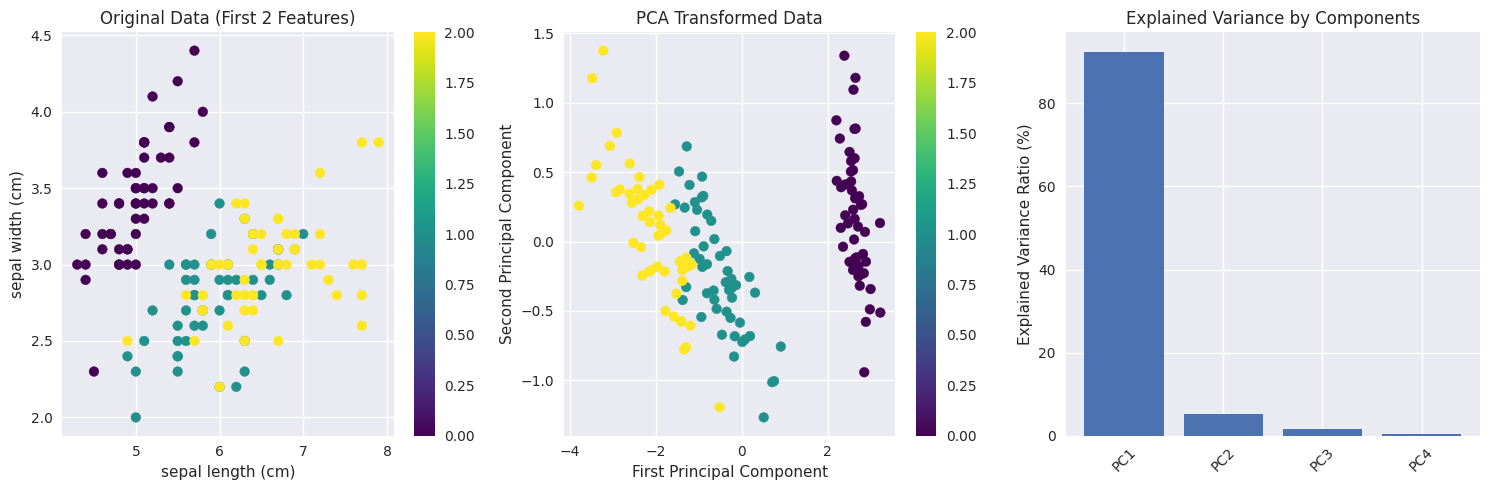
Reconstruction Error Analysis
Source
# Analyze reconstruction error for different numbers of components
n_features = X_iris.shape[1]
reconstruction_errors = []

for n_comp in range(1, n_features + 1):
    X_pca_temp, components_temp, _, mean_temp = pca_from_scratch(X_iris, n_comp)
    X_reconstructed = reconstruct_data(X_pca_temp, components_temp, mean_temp)

    # Calculate mean squared error
    mse = np.mean((X_iris - X_reconstructed) ** 2)
    reconstruction_errors.append(mse)

plt.figure(figsize=(10, 6))
plt.plot(range(1, n_features + 1), reconstruction_errors, 'bo-')
plt.xlabel('Number of Principal Components')
plt.ylabel('Mean Squared Reconstruction Error')
plt.title('Reconstruction Error vs Number of Components')
plt.grid(True, alpha=0.3)
plt.xticks(range(1, n_features + 1))

for i, error in enumerate(reconstruction_errors):
    plt.annotate(f'{error:.4f}', (i+1, error), textcoords="offset points", xytext=(0,10), ha='center')

plt.show()

print("Reconstruction errors:")
for i, error in enumerate(reconstruction_errors):
    print(f"{i+1} components: MSE = {error:.6f}")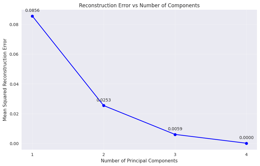
Reconstruction errors:
1 components: MSE = 0.085604
2 components: MSE = 0.025341
3 components: MSE = 0.005919
4 components: MSE = 0.000000
High-Dimensional Data Example
Source
# Generate high-dimensional data with intrinsic low-dimensional structure
np.random.seed(42)
n_samples = 200
n_features = 50
n_informative = 3  # True dimensionality

# Generate data with only 3 informative dimensions
X_high_dim = np.random.randn(n_samples, n_informative)

# Create a random mixing matrix to embed in high-dimensional space
mixing_matrix = np.random.randn(n_informative, n_features)
X_mixed = X_high_dim @ mixing_matrix

# Add some noise
noise_level = 0.1
X_noisy = X_mixed + noise_level * np.random.randn(n_samples, n_features)

print(f"Generated data shape: {X_noisy.shape}")
print(f"True intrinsic dimensionality: {n_informative}")

# Apply PCA
X_pca_high, components_high, eigenvalues_high, mean_high = pca_from_scratch(X_noisy, n_components=10)

# Calculate cumulative explained variance
total_var_high = eigenvalues_high.sum()
explained_var_ratio_high = eigenvalues_high / total_var_high
cumulative_var = np.cumsum(explained_var_ratio_high)

print(f"\nExplained variance by first 10 components:")
for i in range(10):
    print(f"PC{i+1}: {explained_var_ratio_high[i]:.3f} (cumulative: {cumulative_var[i]:.3f})")
Generated data shape: (200, 50)
True intrinsic dimensionality: 3
Explained variance by first 10 components:
PC1: 0.420 (cumulative: 0.420)
PC2: 0.342 (cumulative: 0.763)
PC3: 0.234 (cumulative: 0.997)
PC4: 0.000 (cumulative: 0.997)
PC5: 0.000 (cumulative: 0.997)
PC6: 0.000 (cumulative: 0.997)
PC7: 0.000 (cumulative: 0.997)
PC8: 0.000 (cumulative: 0.998)
PC9: 0.000 (cumulative: 0.998)
PC10: 0.000 (cumulative: 0.998)
Source
# Visualize the explained variance
plt.figure(figsize=(12, 5))

# Plot 1: Individual explained variance
plt.subplot(1, 2, 1)
plt.bar(range(1, 11), explained_var_ratio_high[:10] * 100)
plt.xlabel('Principal Component')
plt.ylabel('Explained Variance Ratio (%)')
plt.title('Individual Explained Variance')
plt.xticks(range(1, 11))

# Plot 2: Cumulative explained variance
plt.subplot(1, 2, 2)
plt.plot(range(1, 11), cumulative_var[:10] * 100, 'bo-')
plt.axhline(y=95, color='r', linestyle='--', label='95% threshold')
plt.xlabel('Number of Components')
plt.ylabel('Cumulative Explained Variance (%)')
plt.title('Cumulative Explained Variance')
plt.legend()
plt.grid(True, alpha=0.3)
plt.xticks(range(1, 11))

plt.tight_layout()
plt.show()

# Find number of components for 95% variance
n_components_95 = np.argmax(cumulative_var >= 0.95) + 1
print(f"\nNumber of components needed for 95% variance: {n_components_95}")
print(f"This is close to the true intrinsic dimensionality of {n_informative}")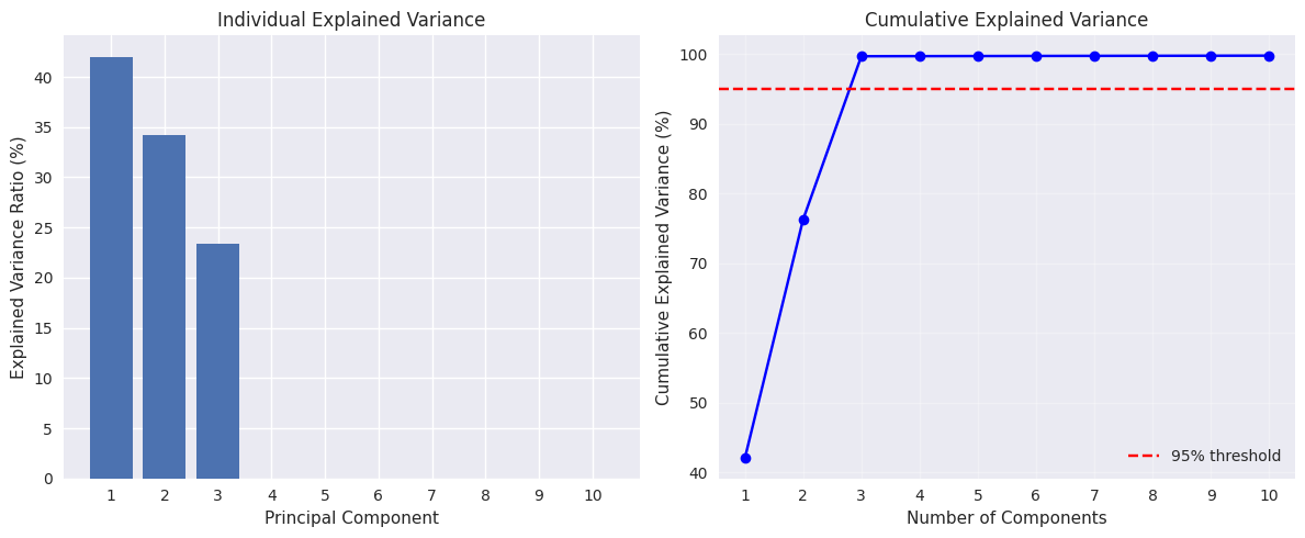
Number of components needed for 95% variance: 3
This is close to the true intrinsic dimensionality of 3
Comparison with Scikit-learn
Source
# Compare our implementation with scikit-learn
from sklearn.decomposition import PCA as SklearnPCA

# Our implementation
X_pca_ours, components_ours, eigenvalues_ours, mean_ours = pca_from_scratch(X_iris, n_components=2)

# Scikit-learn implementation
pca_sklearn = SklearnPCA(n_components=2)
X_pca_sklearn = pca_sklearn.fit_transform(X_iris)

print("Comparison of implementations:")
print(f"Our explained variance ratio: {eigenvalues_ours[:2]/eigenvalues_ours.sum()}")
print(f"Sklearn explained variance ratio: {pca_sklearn.explained_variance_ratio_}")

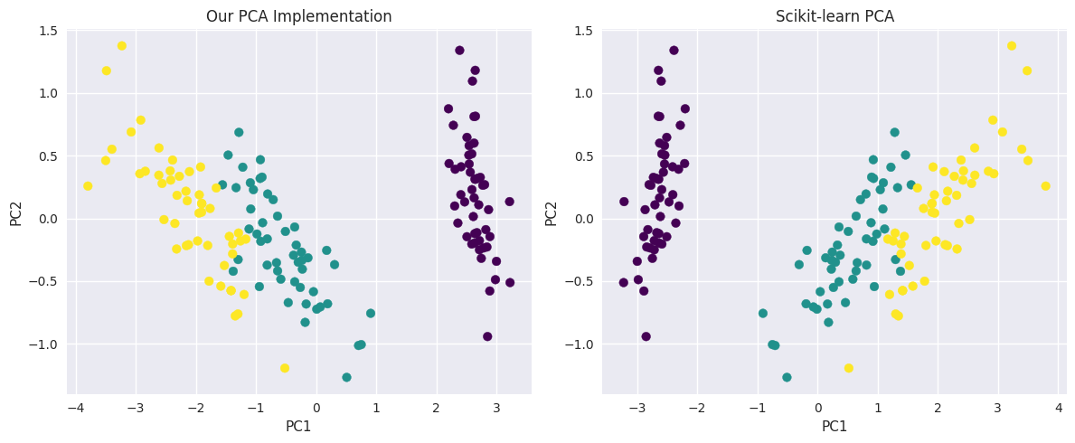
# The signs of eigenvectors might be different, but the results should be equivalent
print(f"\nMean absolute difference in transformed data: {np.mean(np.abs(np.abs(X_pca_ours) - np.abs(X_pca_sklearn))):.10f}")

# Visualize both results
plt.figure(figsize=(12, 5))

plt.subplot(1, 2, 1)
plt.scatter(X_pca_ours[:, 0], X_pca_ours[:, 1], c=y_iris, cmap='viridis')
plt.title('Our PCA Implementation')
plt.xlabel('PC1')
plt.ylabel('PC2')

plt.subplot(1, 2, 2)
plt.scatter(X_pca_sklearn[:, 0], X_pca_sklearn[:, 1], c=y_iris, cmap='viridis')
plt.title('Scikit-learn PCA')
plt.xlabel('PC1')
plt.ylabel('PC2')

plt.tight_layout()
plt.show()
Comparison of implementations:
Our explained variance ratio: [0.92461872 0.05306648]
Sklearn explained variance ratio: [0.92461872 0.05306648]
Mean absolute difference in transformed data: 0.0000000000
Some of my previous papers are about PCA, including Amintoosi & Farbiz (2022)Fathy et al. (2008)Amintoosi et al. (2007)Amintoosi & Poursadeghi (1394)
Summary
This tutorial covered:
Linear Algebra Foundations: Vector operations, norms, and angles
Vector Projections: Mathematical foundation for dimensionality reduction
Basis Transformation: How to represent data in different coordinate systems
PCA Theory: Variance maximization and eigenvalue decomposition
Implementation: Step-by-step PCA algorithm from scratch
Applications: Real examples with Iris dataset and high-dimensional data
Key Takeaways:
PCA finds directions of maximum variance in the data
Principal components are eigenvectors of the covariance matrix
The eigenvalues represent the amount of variance captured by each component
PCA provides optimal linear dimensionality reduction in terms of reconstruction error
The number of components can be chosen based on desired explained variance threshold
- Amintoosi, M., & Farbiz, F. (2022). Eigenbackground Revisited: Can We Model the Background with Eigenvectors? Journal of Mathematical Imaging and Vision, 64(5), 463–477.
- Fathy, M., Mozayani, N., & Amintoosi, M. (2008). Outlier Removal for Super-Resolution Problem Using QR-Decomposition. Proceedings of the International Conference on Image Processing, Computer Vision, and Pattern Recognition, 271–277. http://webpages.iust.ac.ir/mamintoosi/papers/IPCV08.pdf
- Amintoosi, M., Farbiz, F., & Fathy, M. (2007). A QR Decomposition Based Mixture Model Algorithm for Background Modeling. ICICS2007, Sixth International Conference on Information, Communication and Signal Processing, 1–5.
- Amintoosi, M., & Poursadeghi, S. (1394, February). Increasing the Speed of Video Background Subtraction by Incremental QR Decomposition. 8th National Seminar on Linear Algebra and Its Applications.