Kernel Regression: From Linear to Nonlinear Modeling#
1. Linear Regression Foundation#
The goal of regression is to predict a continuous output \(y\) from input features \(\mathbf{x} = (x_0, x_1, ..., x_d)^T\) using a learned function \(f\):
where \(\varepsilon\) is noise. In linear regression, we assume:
The parameters \(\mathbf{w}\) and \(b\) are found by minimizing the sum of squared errors (SSE):
2. Kernel Regression: Nonlinear Extension#
2.1 Intuition#
When relationships are nonlinear, we map inputs \(\mathbf{x}\) to a high-dimensional space \(\phi(\mathbf{x})\) where linear regression operates:
Key Idea: Instead of computing \(\phi(\mathbf{x})\) explicitly, use a kernel function \(K(\mathbf{x}_i, \mathbf{x}_j) = \langle \phi(\mathbf{x}_i), \phi(\mathbf{x}_j) \rangle\).
2.2 Mathematical Formulation#
The kernel regression estimator is a weighted average of training outputs:
where weights \(\alpha_i\) are learned by solving:
In matrix form with kernel matrix \(\mathbf{K}_{ij} = K(\mathbf{x}_i, \mathbf{x}_j)\):
Regularized version (for numerical stability):
3. Primal vs. Dual Perspective#
3.1 Primal Form (Explicit Feature Space)#
Requires explicit \(\phi(\mathbf{x})\) computation
Suitable when feature space dimension is manageable
3.2 Dual Form (Kernel Trick)#
Only requires kernel evaluations
Enables infinite-dimensional feature spaces
Equivalence: For invertible \(\mathbf{K}\), both forms yield identical predictions.
4. Common Kernels#
Kernel Type |
Formula |
Properties |
|---|---|---|
Linear |
\(K(\mathbf{x}, \mathbf{z}) = \mathbf{x}^T \mathbf{z}\) |
Equivalent to linear regression |
Polynomial |
\(K(\mathbf{x}, \mathbf{z}) = (\mathbf{x}^T \mathbf{z} + c)^d\) |
Captures polynomial interactions |
RBF (Gaussian) |
\(K(\mathbf{x}, \mathbf{z}) = \exp\left(-\gamma |\mathbf{x} - \mathbf{z}|^2\right)\) |
Local smoothing, universal approximator |
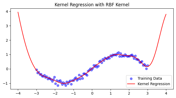
5. Practical Implementation#
import numpy as np
from sklearn.metrics.pairwise import rbf_kernel
import matplotlib.pyplot as plt

# Generate synthetic data
X = np.linspace(-3, 3, 100)[:, None]
y = np.sin(X).ravel() + 0.1*np.random.randn(100)

# Compute RBF kernel (σ=1.0)
K = rbf_kernel(X, X, gamma=0.5)

# Solve for coefficients (with small regularization)
alpha = np.linalg.solve(K + 1e-6*np.eye(len(X)), y)

# Predict new points
X_test = np.linspace(-4, 4, 200)[:, None]
K_test = rbf_kernel(X_test, X, gamma=0.5)
y_pred = K_test @ alpha

# Plot results
plt.figure(figsize=(8, 4))
plt.scatter(X, y, color='blue', label='Training Data', alpha=0.5)
plt.plot(X_test, y_pred, color='red', label='Kernel Regression')
plt.title('Kernel Regression with RBF Kernel')
plt.legend()
plt.show()
6. Key Takeaways#
Nonlinearity via Kernels: Maps data implicitly to high-dimensional spaces
Computational Efficiency: Avoids explicit feature computation via the kernel trick
Flexibility: Kernel choice controls model complexity (RBF for smooth functions, polynomial for interactions)
Regularization: Essential for numerical stability when \(\mathbf{K}\) is ill-conditioned
Matrix Formulation and Primal-Dual Equivalence in Kernel Regression#
1. Primal vs. Dual Matrix Forms#
In linear regression, the weight vector \(\mathbf{w}\) can be estimated in two equivalent ways:
Primal Form (Feature Space):
\[ \mathbf{w} = (\mathbf{X}^T \mathbf{X})^{-1} \mathbf{X}^T \mathbf{y} \]Requires inversion of \(\mathbf{X}^T \mathbf{X} \in \mathbb{R}^{d \times d}\)
Computationally expensive for high-dimensional features (\(d \gg n\))
Dual Form (Sample Space):
\[ \mathbf{w} = \mathbf{X}^T (\mathbf{X} \mathbf{X}^T)^{-1} \mathbf{y} \]Inverts \(\mathbf{X} \mathbf{X}^T \in \mathbb{R}^{n \times n}\) (efficient when \(n \ll d\))
Reveals \(\mathbf{w}\) as a linear combination of samples: \(\mathbf{w} = \sum_{i=1}^n \alpha_i \mathbf{x}_i\)
2. Proof of Equivalence#
For any matrix \(\mathbf{X} \in \mathbb{R}^{n \times d}\) with full row/column rank and \(\lambda > 0\):
Key Steps:
Multiply both sides by \((\mathbf{X}^T \mathbf{X} + \lambda \mathbf{I}_d)\):
\[ \mathbf{X}^T = \mathbf{X}^T (\mathbf{X} \mathbf{X}^T + \lambda \mathbf{I}_n)^{-1} (\mathbf{X} \mathbf{X}^T + \lambda \mathbf{I}_n) \]Simplifies to \(\mathbf{X}^T = \mathbf{X}^T\).
Intuition: Both sides are left inverses of \(\mathbf{X}\) when \(\lambda = 0\) (for invertible \(\mathbf{X}\)).
Special Case (\(\lambda = 0\)):
Holds only if \(\mathbf{X}\) is full-rank (otherwise, pseudo-inverses are needed).
3. Kernelized Version#
Replace \(\mathbf{X}\) with \(\Phi\) (mapped features) and use the kernel trick \(\Phi \Phi^T = \mathbf{K}\):
Prediction: \(\hat{y} = \sum_{i=1}^n \alpha_i K(\mathbf{x}_i, \mathbf{x})\)
Why This Matters:
Avoids explicit computation of \(\Phi\) (which may be infinite-dimensional, e.g., for RBF kernels)
All operations rely solely on the kernel matrix \(\mathbf{K}\)
4. Practical Implications#
Scenario |
Primal Form |
Dual Form |
|---|---|---|
\(n \ll d\) |
Slow (invert \(d \times d\)) |
Fast (invert \(n \times n\)) |
Nonlinear Kernels |
Not applicable |
Required for kernel trick |
Numerical Stability |
Needs \(\lambda > 0\) |
Needs \(\lambda > 0\) |
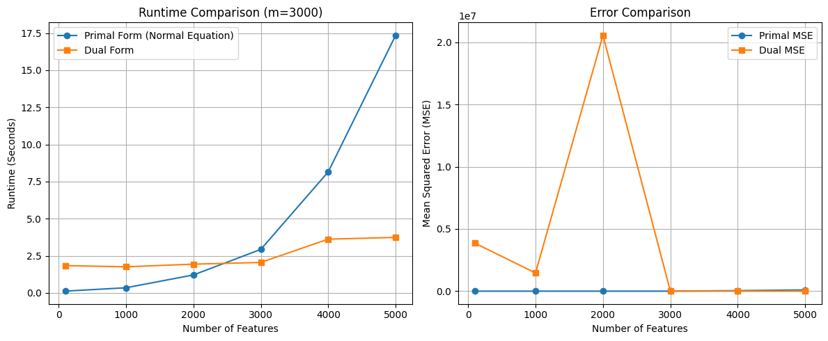
Example: For RBF kernel with \(n=1000\) samples and \(d=10^6\) features:
Primal: Invert \(10^6 \times 10^6\) matrix → Impossible
Dual: Invert \(1000 \times 1000\) kernel matrix → Feasible
5. Numerical Stability Note#
Always add \(\lambda \mathbf{I}\) (ridge penalty) to avoid singular matrices:
alpha = np.linalg.solve(K + 1e-6 * np.eye(n), y)
\(\lambda\) controls the trade-off between stability and overfitting.
Summary: The equivalence \((\mathbf{X}^T \mathbf{X})^{-1} \mathbf{X}^T = \mathbf{X}^T (\mathbf{X} \mathbf{X}^T)^{-1}\) enables flexible, scalable regression via the dual form, which is critical for kernel methods. The kernel trick extends this to nonlinear spaces without explicit feature computation.
References
Bishop, C. Pattern Recognition and Machine Learning (2006)
Comparing Primal and Dual Form#
import numpy as np
import time
import matplotlib.pyplot as plt

# Dataset sizes to test
number_of_features = [100, 1000, 2000, 3000, 4000, 5000]
m = 3000  # Number of instances

primal_times = []
dual_times = []
primal_errors = []
dual_errors = []

for n in number_of_features:
    # Generate dataset
    x = 2 * np.random.rand(m, n)
    y = 4 + 3 * x[:, 0] + np.random.randn(m)
    X = np.c_[np.ones((m, 1)), x]  # Add bias term

    # --- Primal Form (Normal Equation) ---
    start_time = time.time()
    theta_primal = np.linalg.inv(X.T.dot(X)).dot(X.T).dot(y)
    primal_time = time.time() - start_time
    primal_times.append(primal_time)

    # Calculate MSE for Primal
    y_pred_primal = X.dot(theta_primal)
    mse_primal = np.mean((y_pred_primal - y)**2)
    primal_errors.append(mse_primal)

    # --- Dual Form ---
    start_time = time.time()
    theta_dual = X.T.dot(np.linalg.inv(X.dot(X.T)).dot(y))
    dual_time = time.time() - start_time
    dual_times.append(dual_time)

    # Calculate MSE for Dual
    y_pred_dual = X.dot(theta_dual)
    mse_dual = np.mean((y_pred_dual - y)**2)
    dual_errors.append(mse_dual)

# --- Plot Runtime Comparison ---
plt.figure(figsize=(12, 5))
plt.subplot(1, 2, 1)
plt.plot(number_of_features, primal_times, 'o-', label="Primal Form (Normal Equation)")
plt.plot(number_of_features, dual_times, 's-', label="Dual Form")
plt.xlabel("Number of Features")
plt.ylabel("Runtime (Seconds)")
plt.title(f"Runtime Comparison (m={m})")
plt.legend()
plt.grid(True)

# --- Plot Error Comparison ---
plt.subplot(1, 2, 2)
plt.plot(number_of_features, primal_errors, 'o-', label="Primal MSE")
plt.plot(number_of_features, dual_errors, 's-', label="Dual MSE")
plt.xlabel("Number of Features")
plt.ylabel("Mean Squared Error (MSE)")
plt.title("Error Comparison")
plt.legend()
plt.grid(True)

plt.tight_layout()
plt.show()
Appendix#
Proof that \((X^T X)^{-1} X^T = X^T (X X^T)^{-1}\) when \(X\) is a real matrix with full column rank.
Let \(X\) be an \(n \times d\) matrix with \(n \geq d\) and full column rank.
Start with the right-hand side:
Multiply both sides by \(X X^T\):
Now, consider the left-hand side:
But \(X^T X\) is invertible, so:\((X^T X)^{-1} X^T X = I\)
So:
Therefore,