
Ensemble Learning#
Crowd intelligence
Mahmood Amintoosi, Spring 2025
Computer Science Dept, Ferdowsi University of Mashhad
I should mention that the original material of this course was from Open Machine Learning Course, by Joaquin Vanschoren and others.
Show code cell source
# Auto-setup when running on Google Colab
import os
if 'google.colab' in str(get_ipython()) and not os.path.exists('/content/machine-learning'):
    !git clone -q https://github.com/fum-cs/machine-learning.git /content/machine-learning
    !pip --quiet install -r /content/machine-learning/requirements_colab.txt
    %cd machine-learning/notebooks

# Global imports and settings
%matplotlib inline
from preamble import *
interactive = True # Set to True for interactive plots
if interactive:
    fig_scale = 0.9
    plt.rcParams.update(print_config)
else: # For printing
    fig_scale = 0.3
    plt.rcParams.update(print_config)
Ensemble learning#
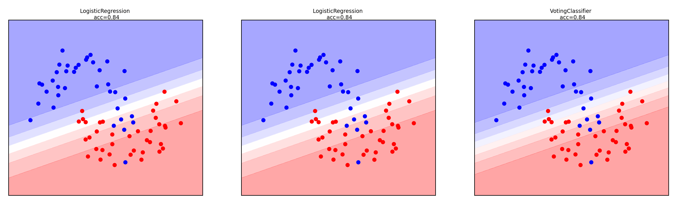
If different models make different mistakes, can we simply average the predictions?
Voting Classifier: gives every model a vote on the class label
Hard vote: majority class wins (class order breaks ties)
Soft vote: sum class probabilities \(p_{m,c}\) over \(M\) models: \(\underset{c}{\operatorname{argmax}} \sum_{m=1}^{M} w_c p_{m,c}\)
Classes can get different weights \(w_c\) (default: \(w_c=1\))
Show code cell source
from sklearn.model_selection import train_test_split
from sklearn.linear_model import LogisticRegression
from sklearn.ensemble import VotingClassifier
from sklearn.neighbors import KNeighborsClassifier
from sklearn.tree import DecisionTreeClassifier
from sklearn.datasets import make_moons
import ipywidgets as widgets
from ipywidgets import interact, interact_manual

# Toy data
X, y = make_moons(noise=.2, random_state=18) # carefully picked random state for illustration
X_train, X_test, y_train, y_test = train_test_split(X, y, stratify=y, random_state=0)

# Plot grid
x_lin = np.linspace(X_train[:, 0].min() - .5, X_train[:, 0].max() + .5, 100)
y_lin = np.linspace(X_train[:, 1].min() - .5, X_train[:, 1].max() + .5, 100)
x_grid, y_grid = np.meshgrid(x_lin, y_lin)
X_grid = np.c_[x_grid.ravel(), y_grid.ravel()]
models = [LogisticRegression(C=100),
          DecisionTreeClassifier(max_depth=3, random_state=0),
          KNeighborsClassifier(n_neighbors=1),
          KNeighborsClassifier(n_neighbors=30)]

@interact
def combine_voters(model1=models, model2=models):
    # Voting Classifier and components
    voting = VotingClassifier([('model1', model1),('model2', model2)],voting='soft')
    voting.fit(X_train, y_train)

    # transform produces individual probabilities
    y_probs =  voting.transform(X_grid)

    fig, axes = plt.subplots(1, 3, subplot_kw={'xticks': (()), 'yticks': (())}, figsize=(11*fig_scale, 3*fig_scale))
    scores = [voting.estimators_[0].score(X_test, y_test),
             voting.estimators_[1].score(X_test, y_test),
             voting.score(X_test, y_test)]
    titles = [model1.__class__.__name__, model2.__class__.__name__, 'VotingClassifier']
    for prob, score, title, ax in zip([y_probs[:, 1], y_probs[:, 3], y_probs[:, 1::2].sum(axis=1)], scores, titles, axes.ravel()):
        ax.contourf(x_grid, y_grid, prob.reshape(x_grid.shape), alpha=.4, cmap='bwr')
        ax.scatter(X_train[:, 0], X_train[:, 1], c=y_train, cmap='bwr', s=7*fig_scale)
        ax.set_title(title + f" \n acc={score:.2f}", pad=0)
Show code cell source
if not interactive:
    combine_voters(models[0],models[1])
Why does this work?
Different models may be good at different ‘parts’ of data (even if they underfit)
Individual mistakes can be ‘averaged out’ (especially if models overfit)
Which models should be combined?
Bias-variance analysis teaches us that we have two options:
If model underfits (high bias, low variance): combine with other low-variance models
Need to be different: ‘experts’ on different parts of the data
Bias reduction. Can be done with Boosting
If model overfits (low bias, high variance): combine with other low-bias models
Need to be different: individual mistakes must be different
Variance reduction. Can be done with Bagging
Models must be uncorrelated but good enough (otherwise the ensemble is worse)
We can also learn how to combine the predictions of different models: Stacking
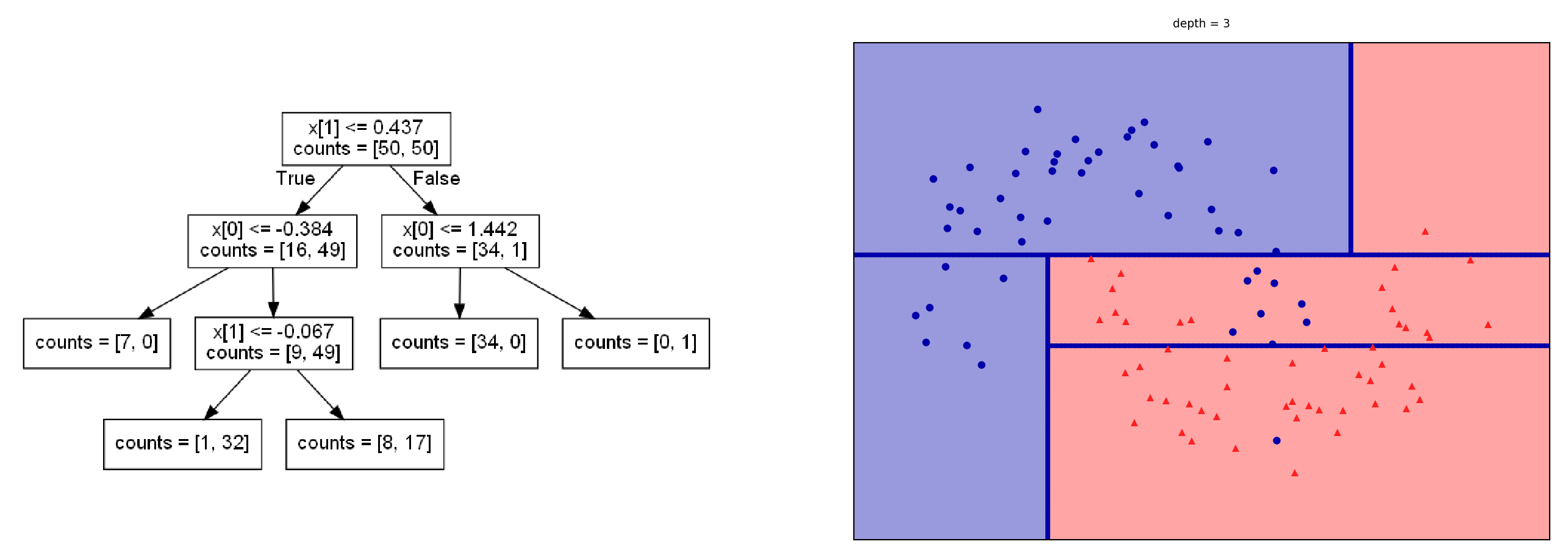
Decision trees (recap)#
Representation: Tree that splits data points into leaves based on tests
Evaluation (loss): Heuristic for purity of leaves (Gini index, entropy,…)
Optimization: Recursive, heuristic greedy search (Hunt’s algorithm)
Consider all splits (thresholds) between adjacent data points, for every feature
Choose the one that yields the purest leafs, repeat
Show code cell source
import graphviz

@interact
def plot_depth(depth=(1,5,1)):
    X, y = make_moons(noise=.2, random_state=18) # carefully picked random state for illustration
    fig, ax = plt.subplots(1, 2, figsize=(12*fig_scale, 4*fig_scale),
                           subplot_kw={'xticks': (), 'yticks': ()})

    tree = mglearn.plots.plot_tree(X, y, max_depth=depth)
    ax[0].imshow(mglearn.plots.tree_image(tree))
    ax[0].set_axis_off()
Show code cell source
if not interactive:
    plot_depth(depth=3)
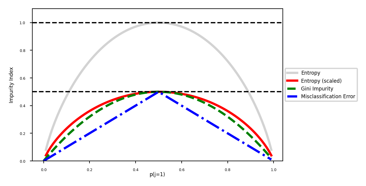
Evaluation (loss function for classification)#
Every leaf predicts a class probability \(\hat{p}_c\) = the relative frequency of class \(c\)
Leaf impurity measures (splitting criteria) for \(L\) leafs, leaf \(l\) has data \(X_l\):
Gini-Index: \(Gini(X_{l}) = \sum_{c\neq c'} \hat{p}_c \hat{p}_{c'}\)
Entropy (more expensive): \(E(X_{l}) = -\sum_{c\neq c'} \hat{p}_c \log_{2}\hat{p}_c\)
Best split maximizes information gain (idem for Gini index) $\( Gain(X,X_i) = E(X) - \sum_{l=1}^L \frac{|X_{i=l}|}{|X_{i}|} E(X_{i=l}) \)$
Show code cell source
def gini(p):
   return (p)*(1 - (p)) + (1 - p)*(1 - (1-p))

def entropy(p):
   return - p*np.log2(p) - (1 - p)*np.log2((1 - p))

def classification_error(p):
   return 1 - np.max([p, 1 - p])

x = np.arange(0.0, 1.0, 0.01)
ent = [entropy(p) if p != 0 else None for p in x]
scaled_ent = [e*0.5 if e else None for e in ent]
c_err = [classification_error(i) for i in x]

fig = plt.figure(figsize=(5*fig_scale, 2.5*fig_scale))
ax = plt.subplot(111)

for j, lab, ls, c, in zip(
      [ent, scaled_ent, gini(x), c_err],
      ['Entropy', 'Entropy (scaled)', 'Gini Impurity', 'Misclassification Error'],
      ['-', '-', '--', '-.'],
      ['lightgray', 'red', 'green', 'blue']):
   line = ax.plot(x, j, label=lab, linestyle=ls, lw=2*fig_scale, color=c)

ax.legend(loc='upper left', ncol=1, fancybox=True, shadow=False)
ax.axhline(y=0.5, linewidth=1, color='k', linestyle='--')
ax.axhline(y=1.0, linewidth=1, color='k', linestyle='--')
box = ax.get_position()
ax.set_position([box.x0, box.y0, box.width * 0.8, box.height])
ax.legend(loc='center left', bbox_to_anchor=(1, 0.5))

plt.ylim([0, 1.1])
plt.xlabel('p(j=1)',labelpad=0)
plt.ylabel('Impurity Index')
plt.show()
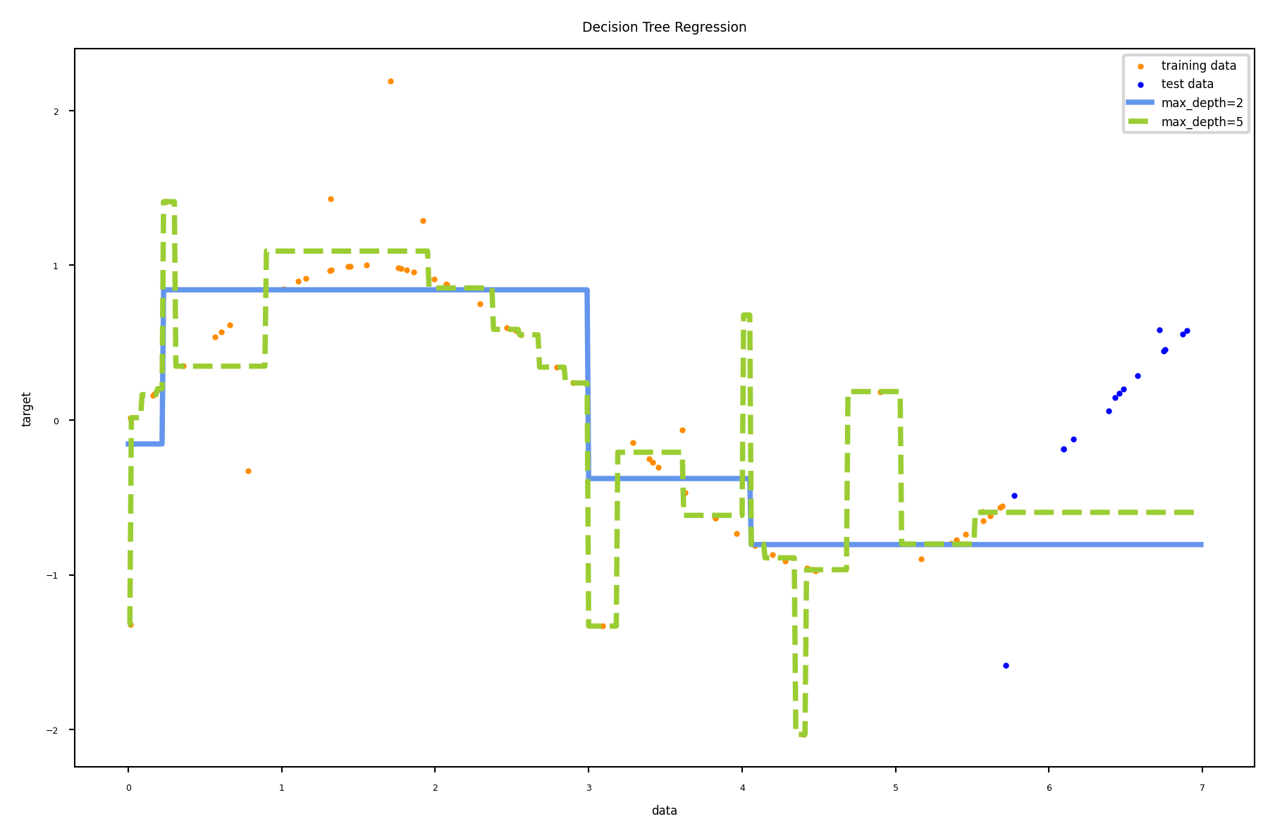
Regression trees#
Every leaf predicts the mean target value \(\mu\) of all points in that leaf
Choose the split that minimizes squared error of the leaves: \(\sum_{x_{i} \in L} (y_i - \mu)^2\)
Yields non-smooth step-wise predictions, cannot extrapolate
Show code cell source
from sklearn.tree import DecisionTreeRegressor

def plot_decision_tree_regression(regr_1, regr_2):
    # Create a random dataset
    rng = np.random.RandomState(5)
    X = np.sort(7 * rng.rand(80, 1), axis=0)
    y = np.sin(X).ravel()
    y[::5] += 3 * (0.5 - rng.rand(16))
    split = 65

    # Fit regression model of first 60 points
    regr_1.fit(X[:split], y[:split])
    regr_2.fit(X[:split], y[:split])

    # Predict
    X_test = np.arange(0.0, 7.0, 0.01)[:, np.newaxis]
    y_1 = regr_1.predict(X_test)
    y_2 = regr_2.predict(X_test)

    # Plot the results
    plt.figure(figsize=(8*fig_scale,5*fig_scale))
    plt.scatter(X[:split], y[:split], c="darkorange", label="training data")
    plt.scatter(X[split:], y[split:], c="blue", label="test data")
    plt.plot(X_test, y_1, color="cornflowerblue", label="max_depth=2", linewidth=2*fig_scale)
    plt.plot(X_test, y_2, color="yellowgreen", label="max_depth=5", linewidth=2*fig_scale)
    plt.xlabel("data")
    plt.ylabel("target")
    plt.title("Decision Tree Regression")
    plt.legend()
    plt.show()

regr_1 = DecisionTreeRegressor(max_depth=2)
regr_2 = DecisionTreeRegressor(max_depth=5)

plot_decision_tree_regression(regr_1,regr_2)
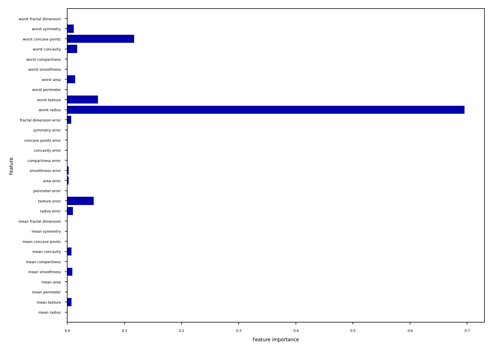
Impurity/Entropy-based feature importance#
We can measure the importance of features (to the model) based on
Which features we split on
How high up in the tree we split on them (first splits ar emore important)
Show code cell source
from sklearn.datasets import load_breast_cancer
cancer = load_breast_cancer()
Xc_train, Xc_test, yc_train, yc_test = train_test_split(cancer.data, cancer.target, stratify=cancer.target, random_state=42)
tree = DecisionTreeClassifier(random_state=0).fit(Xc_train, yc_train)

def plot_feature_importances_cancer(model):
    n_features = cancer.data.shape[1]
    plt.figure(figsize=(7*fig_scale,5.4*fig_scale))
    plt.barh(range(n_features), model.feature_importances_, align='center')
    plt.yticks(np.arange(n_features), cancer.feature_names)
    plt.xlabel("Feature importance")
    plt.ylabel("Feature")
    plt.ylim(-1, n_features)
plot_feature_importances_cancer(tree)
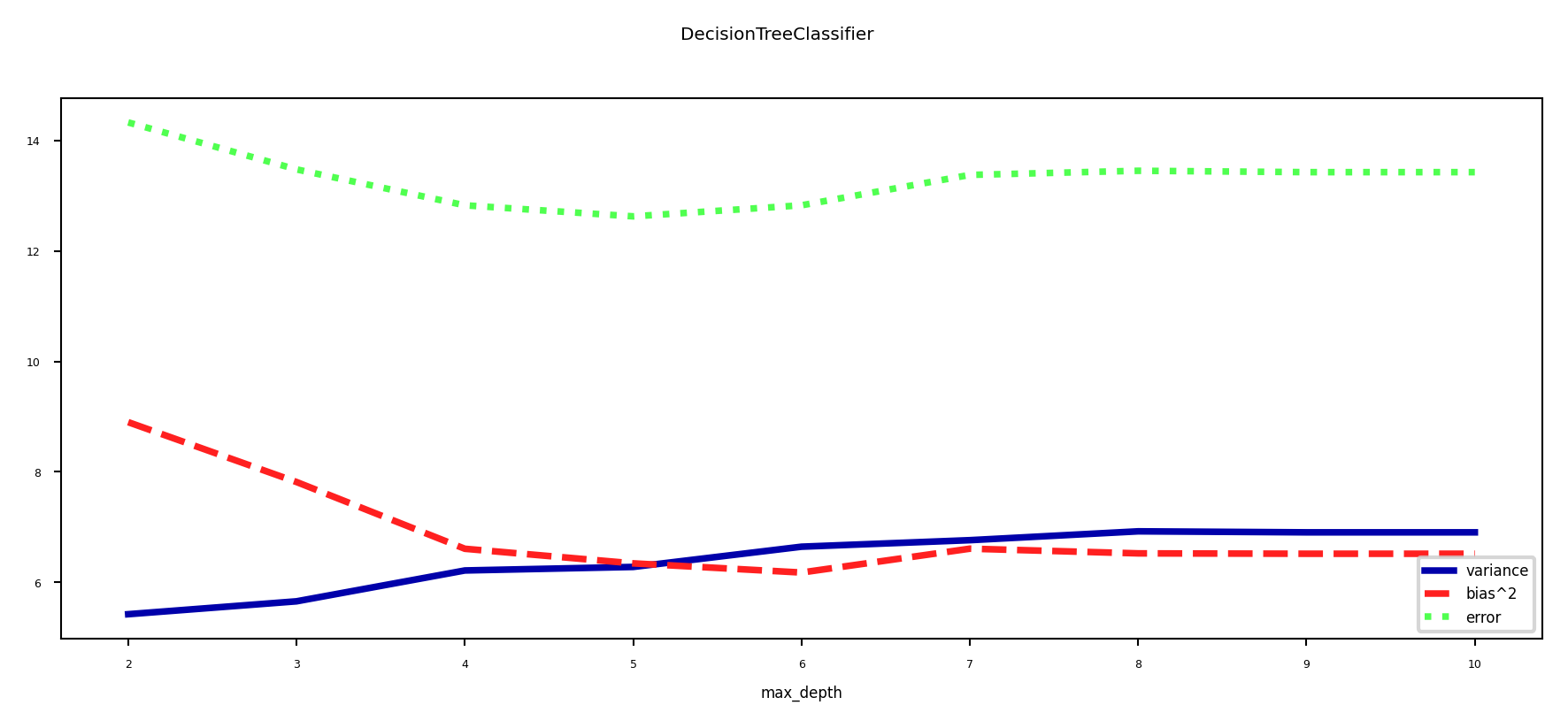
Under- and overfitting#
We can easily control the (maximum) depth of the trees as a hyperparameter
Bias-variance analysis:
Shallow trees have high bias but very low variance (underfitting)
Deep trees have high variance but low bias (overfitting)
Because we can easily control their complexity, they are ideal for ensembling
Deep trees: keep low bias, reduce variance with Bagging
Shallow trees: keep low variance, reduce bias with Boosting
Show code cell source
from sklearn.model_selection import ShuffleSplit, train_test_split

# Bias-Variance Computation
def compute_bias_variance(clf, X, y):
    # Bootstraps
    n_repeat = 40 # 40 is on the low side to get a good estimate. 100 is better.
    shuffle_split = ShuffleSplit(test_size=0.33, n_splits=n_repeat, random_state=0)

    # Store sample predictions
    y_all_pred = [[] for _ in range(len(y))]

    # Train classifier on each bootstrap and score predictions
    for i, (train_index, test_index) in enumerate(shuffle_split.split(X)):
        # Train and predict
        clf.fit(X[train_index], y[train_index])
        y_pred = clf.predict(X[test_index])

        # Store predictions
        for j,index in enumerate(test_index):
            y_all_pred[index].append(y_pred[j])

    # Compute bias, variance, error
    bias_sq = sum([ (1 - x.count(y[i])/len(x))**2 * len(x)/n_repeat
                for i,x in enumerate(y_all_pred)])
    var = sum([((1 - ((x.count(0)/len(x))**2 + (x.count(1)/len(x))**2))/2) * len(x)/n_repeat
               for i,x in enumerate(y_all_pred)])
    error = sum([ (1 - x.count(y[i])/len(x)) * len(x)/n_repeat
            for i,x in enumerate(y_all_pred)])

    return np.sqrt(bias_sq), var, error

def plot_bias_variance(clf, X, y):
    bias_scores = []
    var_scores = []
    err_scores = []
    max_depth= range(2,11)

    for i in max_depth:
        b,v,e = compute_bias_variance(clf.set_params(random_state=0,max_depth=i),X,y)
        bias_scores.append(b)
        var_scores.append(v)
        err_scores.append(e)

    plt.figure(figsize=(8*fig_scale,3*fig_scale))
    plt.suptitle(clf.__class__.__name__)
    plt.plot(max_depth, var_scores,label ="variance", lw=2*fig_scale )
    plt.plot(max_depth, np.square(bias_scores),label ="bias^2", lw=2*fig_scale )
    plt.plot(max_depth, err_scores,label ="error", lw=2*fig_scale)
    plt.xlabel("max_depth")
    plt.legend(loc="best")
    plt.show()

dt = DecisionTreeClassifier()
plot_bias_variance(dt, cancer.data, cancer.target)
Bagging (Bootstrap Aggregating)#
Obtain different models by training the same model on different training samples
Reduce overfitting by averaging out individual predictions (variance reduction)
In practice: take \(I\) bootstrap samples of your data, train a model on each bootstrap
Higher \(I\): more models, more smoothing (but slower training and prediction)
Base models should be unstable: different training samples yield different models
E.g. very deep decision trees, or even randomized decision trees
Deep Neural Networks can also benefit from bagging (deep ensembles)
Prediction by averaging predictions of base models
Soft voting for classification (possibly weighted)
Mean value for regression
Can produce uncertainty estimates as well
By combining class probabilities of individual models (or variances for regression)
Random Forests#
Uses randomized trees to make models even less correlated (more unstable)
At every split, only consider
max_featuresfeatures, randomly selected
Extremely randomized trees: considers 1 random threshold for random set of features (faster)
Show code cell source
from sklearn.ensemble import RandomForestClassifier, ExtraTreesClassifier
from sklearn.datasets import make_moons
from sklearn.model_selection import train_test_split

models=[RandomForestClassifier(n_estimators=5, random_state=7, n_jobs=-1),ExtraTreesClassifier(n_estimators=5, random_state=2, n_jobs=-1)]

@interact
def run_forest_run(model=models):
    forest = model.fit(X_train, y_train)
    fig, axes = plt.subplots(2, 3, figsize=(12*fig_scale, 6*fig_scale))
    for i, (ax, tree) in enumerate(zip(axes.ravel(), forest.estimators_)):
        ax.set_title("Tree {}".format(i), pad=0)
        mglearn.plots.plot_tree_partition(X_train, y_train, tree, ax=ax)

    mglearn.plots.plot_2d_separator(forest, X_train, fill=True, ax=axes[-1, -1],
                                    alpha=.4)
    axes[-1, -1].set_title(model.__class__.__name__, pad=0)
    axes[-1, -1].set_xticks(())
    axes[-1, -1].set_yticks(())
    mglearn.discrete_scatter(X_train[:, 0], X_train[:, 1], y_train, s=10*fig_scale);

Show code cell source
if not interactive:
    run_forest_run(model=models[0])
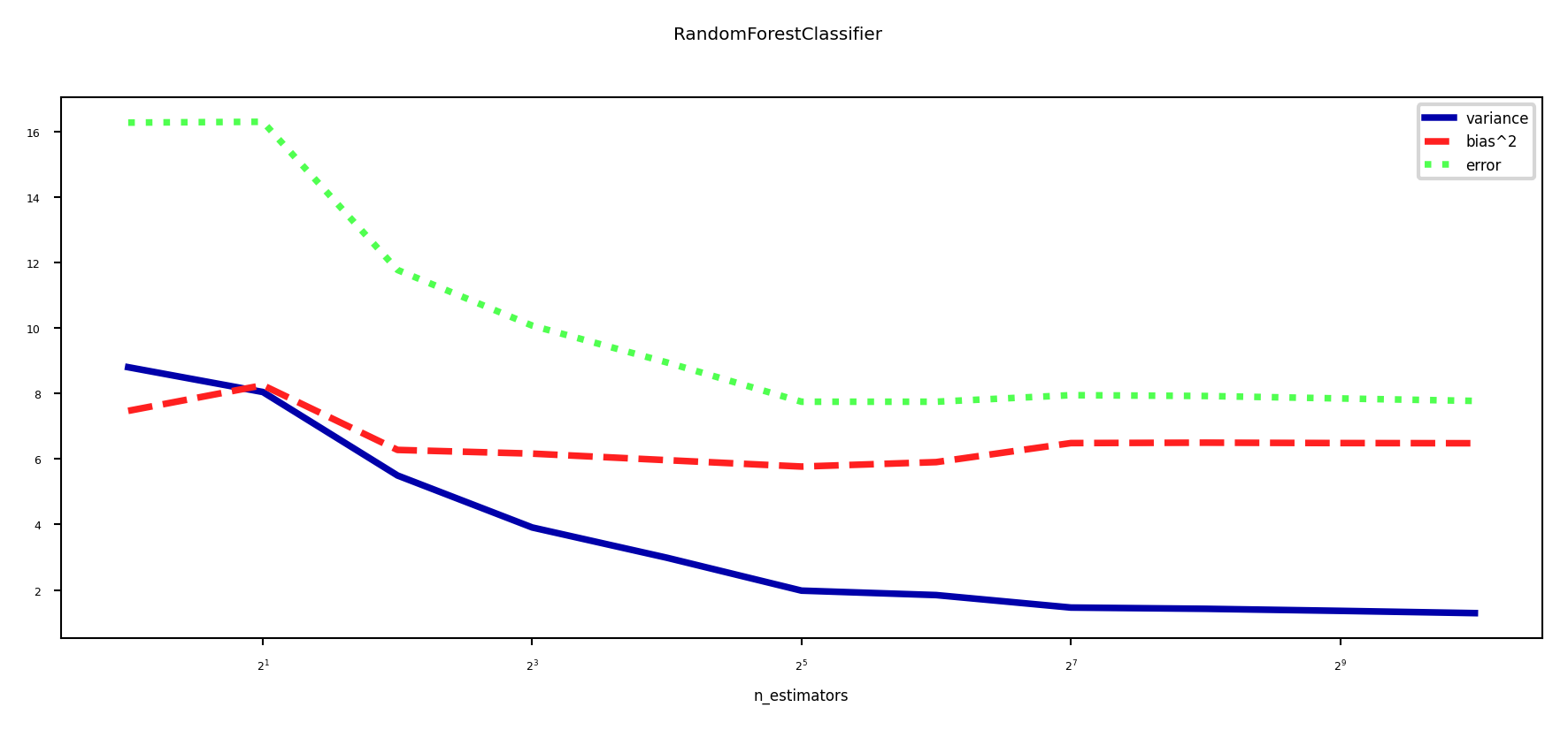
Effect on bias and variance#
Increasing the number of models (trees) decreases variance (less overfitting)
Bias is mostly unaffected, but will increase if the forest becomes too large (oversmoothing)
Show code cell source
from sklearn.model_selection import ShuffleSplit, train_test_split
from sklearn.datasets import load_breast_cancer
from sklearn.ensemble import RandomForestClassifier
cancer = load_breast_cancer()

# Faster version of plot_bias_variance that uses warm-starting
def plot_bias_variance_rf(model, X, y, warm_start=False):
    bias_scores = []
    var_scores = []
    err_scores = []

    # Bootstraps
    n_repeat = 40 # 40 is on the low side to get a good estimate. 100 is better.
    shuffle_split = ShuffleSplit(test_size=0.33, n_splits=n_repeat, random_state=0)

    # Ensemble sizes
    n_estimators = [1, 2, 4, 8, 16, 32, 64, 128, 256, 512, 1024]

    # Store sample predictions. One per n_estimators
    # n_estimators : [predictions]
    predictions = {}
    for nr_trees in n_estimators:
        predictions[nr_trees] = [[] for _ in range(len(y))]

    # Train classifier on each bootstrap and score predictions
    for i, (train_index, test_index) in enumerate(shuffle_split.split(X)):

        # Initialize
        clf = model(random_state=0)
        if model.__class__.__name__ == 'RandomForestClassifier':
            clf.n_jobs = -1
        if model.__class__.__name__ != 'AdaBoostClassifier':
            clf.warm_start = warm_start

        prev_n_estimators = 0

        # Train incrementally
        for nr_trees in n_estimators:
            if model.__class__.__name__ == 'HistGradientBoostingClassifier':
                clf.max_iter = nr_trees
            else:
                clf.n_estimators = nr_trees

            # Fit and predict
            clf.fit(X[train_index], y[train_index])
            y_pred = clf.predict(X[test_index])
            for j,index in enumerate(test_index):
                predictions[nr_trees][index].append(y_pred[j])

    for nr_trees in n_estimators:
        # Compute bias, variance, error
        bias_sq = sum([ (1 - x.count(y[i])/len(x))**2 * len(x)/n_repeat
                       for i,x in enumerate(predictions[nr_trees])])
        var = sum([((1 - ((x.count(0)/len(x))**2 + (x.count(1)/len(x))**2))/2) * len(x)/n_repeat
                   for i,x in enumerate(predictions[nr_trees])])
        error = sum([ (1 - x.count(y[i])/len(x)) * len(x)/n_repeat
                     for i,x in enumerate(predictions[nr_trees])])

        bias_scores.append(bias_sq)
        var_scores.append(var)
        err_scores.append(error)

    plt.figure(figsize=(8*fig_scale,3*fig_scale))
    plt.suptitle(clf.__class__.__name__)
    plt.plot(n_estimators, var_scores,label = "variance", lw=2*fig_scale )
    plt.plot(n_estimators, bias_scores,label = "bias^2", lw=2*fig_scale )
    plt.plot(n_estimators, err_scores,label = "error", lw=2*fig_scale  )
    plt.xscale('log',base=2)
    plt.xlabel("n_estimators")
    plt.legend(loc="best")
    plt.show()
plot_bias_variance_rf(RandomForestClassifier, cancer.data, cancer.target, warm_start=True)
In practice#
Different implementations can be used. E.g. in scikit-learn:
BaggingClassifier: Choose your own base model and sampling procedureRandomForestClassifier: Default implementation, many optionsExtraTreesClassifier: Uses extremely randomized trees
Most important parameters:
n_estimators(>100, higher is better, but diminishing returns)Will start to underfit (bias error component increases slightly)
max_featuresDefaults: \(sqrt(p)\) for classification, \(log2(p)\) for regression
Set smaller to reduce space/time requirements
parameters of trees, e.g.
max_depth,min_samples_split,…Prepruning useful to reduce model size, but don’t overdo it
Easy to parallelize (set
n_jobsto -1)Fix
random_state(bootstrap samples) for reproducibility
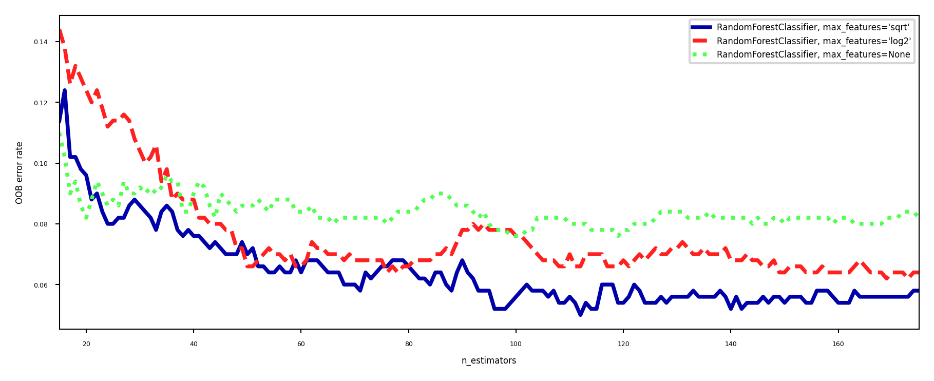
Out-of-bag error#
RandomForests don’t need cross-validation: you can use the out-of-bag (OOB) error
For each tree grown, about 33% of samples are out-of-bag (OOB)
Remember which are OOB samples for every model, do voting over these
OOB error estimates are great to speed up model selection
As good as CV estimates, althought slightly pessimistic
In scikit-learn:
oob_error = 1 - clf.oob_score_
Show code cell source
from collections import OrderedDict
from sklearn.datasets import make_classification
from sklearn.ensemble import RandomForestClassifier, ExtraTreesClassifier

RANDOM_STATE = 123

# Generate a binary classification dataset.
X, y = make_classification(n_samples=500, n_features=25,
                           n_clusters_per_class=1, n_informative=15,
                           random_state=RANDOM_STATE)

# NOTE: Setting the `warm_start` construction parameter to `True` disables
# support for parallelized ensembles but is necessary for tracking the OOB
# error trajectory during training.
ensemble_clfs = [
    ("RandomForestClassifier, max_features='sqrt'",
        RandomForestClassifier(warm_start=True, oob_score=True,
                               max_features="sqrt", n_jobs=-1,
                               random_state=RANDOM_STATE)),
    ("RandomForestClassifier, max_features='log2'",
        RandomForestClassifier(warm_start=True, max_features='log2',
                               oob_score=True, n_jobs=-1,
                               random_state=RANDOM_STATE)),
    ("RandomForestClassifier, max_features=None",
        RandomForestClassifier(warm_start=True, max_features=None,
                               oob_score=True, n_jobs=-1,
                               random_state=RANDOM_STATE))
]

# Map a classifier name to a list of (<n_estimators>, <error rate>) pairs.
error_rate = OrderedDict((label, []) for label, _ in ensemble_clfs)

# Range of `n_estimators` values to explore.
min_estimators = 15
max_estimators = 175

for label, clf in ensemble_clfs:
    for i in range(min_estimators, max_estimators + 1):
        clf.set_params(n_estimators=i)
        clf.fit(X, y)

        # Record the OOB error for each `n_estimators=i` setting.
        oob_error = 1 - clf.oob_score_
        error_rate[label].append((i, oob_error))

# Generate the "OOB error rate" vs. "n_estimators" plot.
plt.figure(figsize=(8*fig_scale,3*fig_scale))
for label, clf_err in error_rate.items():
    xs, ys = zip(*clf_err)
    plt.plot(xs, ys, label=label, lw=2*fig_scale)

plt.xlim(min_estimators, max_estimators)
plt.xlabel("n_estimators")
plt.ylabel("OOB error rate")
plt.legend(loc="upper right")
plt.show()
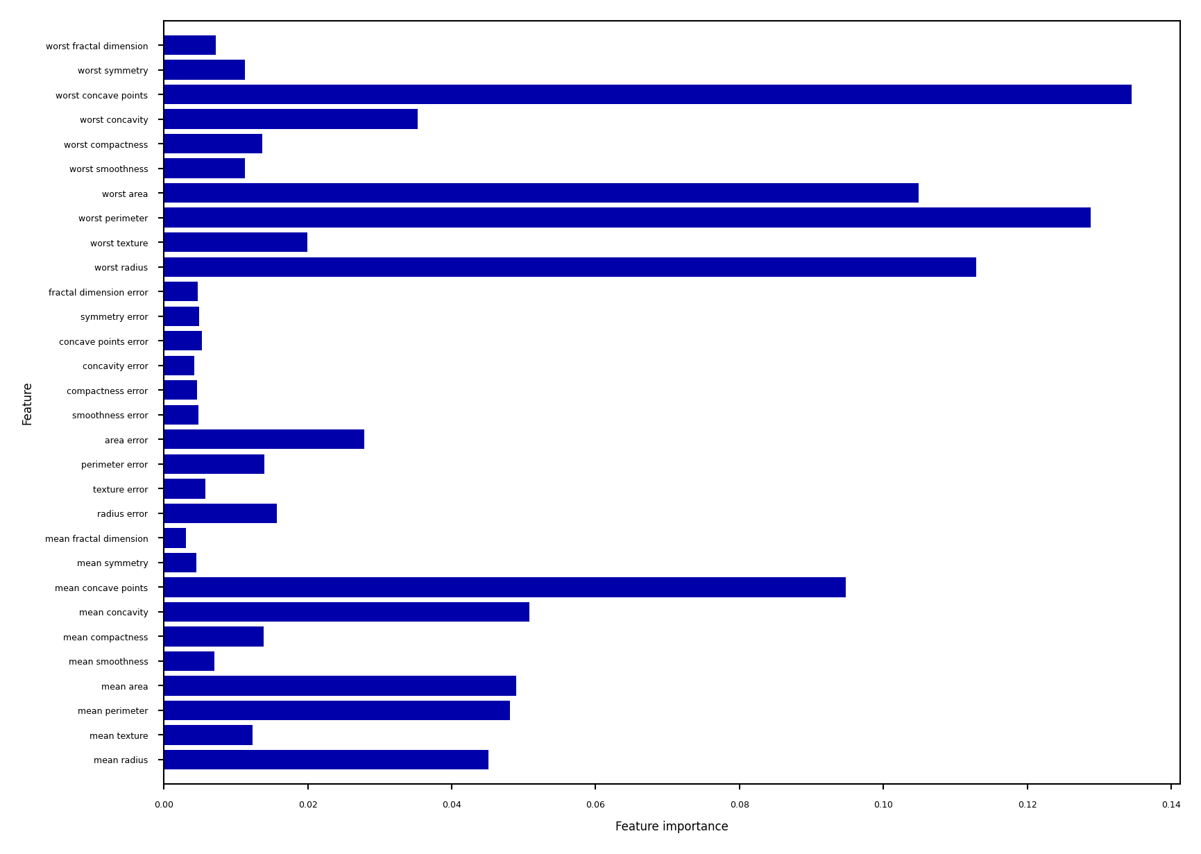
Feature importance#
RandomForests provide more reliable feature importances, based on many alternative hypotheses (trees)
Show code cell source
forest = RandomForestClassifier(random_state=0, n_estimators=512, n_jobs=-1)
forest.fit(Xc_train, yc_train)
plot_feature_importances_cancer(forest)
Other tips#
Model calibration
RandomForests are poorly calibrated.
Calibrate afterwards (e.g. isotonic regression) if you aim to use probabilities
Warm starting
Given an ensemble trained for \(I\) iterations, you can simply add more models later
You warm start from the existing model instead of re-starting from scratch
Can be useful to train models on new, closely related data
Not ideal if the data batches change over time (concept drift)
Boosting is more robust against this (see later)
Strength and weaknesses#
RandomForest are among most widely used algorithms:
Don’t require a lot of tuning
Typically very accurate
Handles heterogeneous features well (trees)
Implictly selects most relevant features
Downsides:
less interpretable, slower to train (but parallellizable)
don’t work well on high dimensional sparse data (e.g. text)
Adaptive Boosting (AdaBoost)#
Obtain different models by reweighting the training data every iteration
Reduce underfitting by focusing on the ‘hard’ training examples
Increase weights of instances misclassified by the ensemble, and vice versa
Base models should be simple so that different instance weights lead to different models
Underfitting models: decision stumps (or very shallow trees)
Each is an ‘expert’ on some parts of the data
Additive model: Predictions at iteration \(I\) are sum of base model predictions
In Adaboost, also the models each get a unique weight \(w_i\) $\(f_I(\mathbf{x}) = \sum_{i=1}^I w_i g_i(\mathbf{x})\)$
Adaboost minimizes exponential loss. For instance-weighted error \(\varepsilon\): $\(\mathcal{L}_{Exp} = \sum_{n=1}^N e^{\varepsilon(f_I(\mathbf{x}))}\)$
By deriving \(\frac{\partial \mathcal{L}}{\partial w_i}\) you can find that optimal \(w_{i} = \frac{1}{2}\log(\frac{1-\varepsilon}{\varepsilon})\)
AdaBoost algorithm#
Initialize sample weights: \(s_{n,0} = \frac{1}{N}\)
Build a model (e.g. decision stumps) using these sample weights
Give the model a weight \(w_i\) related to its weighted error rate \(\varepsilon\) $\(w_{i} = \lambda\log(\frac{1-\varepsilon}{\varepsilon})\)$
Good trees get more weight than bad trees
Logit function maps error \(\varepsilon\) from [0,1] to weight in [-Inf,Inf] (use small minimum error)
Learning rate \(\lambda\) (shrinkage) decreases impact of individual classifiers
Small updates are often better but requires more iterations
Update the sample weights
Increase weight of incorrectly predicted samples: \(s_{n,i+1} = s_{n,i}e^{w_i}\)
Decrease weight of correctly predicted samples: \(s_{n,i+1} = s_{n,i}e^{-w_i}\)
Normalize weights to add up to 1
Repeat for \(I\) iterations
AdaBoost variants#
Discrete Adaboost: error rate \(\varepsilon\) is simply the error rate (1-Accuracy)
Real Adaboost: \(\varepsilon\) is based on predicted class probabilities \(\hat{p}_c\) (better)
AdaBoost for regression: \(\varepsilon\) is either linear (\(|y_i-\hat{y}_i|\)), squared (\((y_i-\hat{y}_i)^2\)), or exponential loss
GentleBoost: adds a bound on model weights \(w_i\)
LogitBoost: Minimizes logistic loss instead of exponential loss $\(\mathcal{L}_{Logistic} = \sum_{n=1}^N log(1+e^{\varepsilon(f_I(\mathbf{x}))})\)$
Adaboost in action#
Size of the samples represents sample weight
Background shows the latest tree’s predictions
Show code cell source
from matplotlib.colors import ListedColormap
from sklearn.tree import DecisionTreeClassifier
import ipywidgets as widgets
from ipywidgets import interact, interact_manual
from sklearn.preprocessing import normalize

# Code adapted from https://xavierbourretsicotte.github.io/AdaBoost.html
def AdaBoost_scratch(X,y, M=10, learning_rate = 0.5):
    #Initialization of utility variables
    N = len(y)
    estimator_list, y_predict_list, estimator_error_list, estimator_weight_list, sample_weight_list = [],[],[],[],[]

    #Initialize the sample weights
    sample_weight = np.ones(N) / N
    sample_weight_list.append(sample_weight.copy())

    #For m = 1 to M
    for m in range(M):

        #Fit a classifier
        estimator = DecisionTreeClassifier(max_depth = 1, max_leaf_nodes=2)
        estimator.fit(X, y, sample_weight=sample_weight)
        y_predict = estimator.predict(X)

        #Misclassifications
        incorrect = (y_predict != y)

        #Estimator error
        estimator_error = np.mean( np.average(incorrect, weights=sample_weight, axis=0))

        #Boost estimator weights
        estimator_weight =  learning_rate * np.log((1. - estimator_error) / estimator_error)

        #Boost sample weights
        sample_weight *= np.exp(estimator_weight * incorrect * ((sample_weight > 0) | (estimator_weight < 0)))
        sample_weight *= np.exp(-estimator_weight * np.invert(incorrect * ((sample_weight > 0) | (estimator_weight < 0))))
        sample_weight /= np.linalg.norm(sample_weight)

        #Save iteration values
        estimator_list.append(estimator)
        y_predict_list.append(y_predict.copy())
        estimator_error_list.append(estimator_error.copy())
        estimator_weight_list.append(estimator_weight.copy())
        sample_weight_list.append(sample_weight.copy())

    #Convert to np array for convenience
    estimator_list = np.asarray(estimator_list)
    y_predict_list = np.asarray(y_predict_list)
    estimator_error_list = np.asarray(estimator_error_list)
    estimator_weight_list = np.asarray(estimator_weight_list)
    sample_weight_list = np.asarray(sample_weight_list)

    #Predictions
    preds = (np.array([np.sign((y_predict_list[:,point] * estimator_weight_list).sum()) for point in range(N)]))
    #print('Accuracy = ', (preds == y).sum() / N)

    return estimator_list, estimator_weight_list, sample_weight_list, estimator_error_list

def plot_decision_boundary(classifier, X, y, N = 10, scatter_weights = np.ones(len(y)) , ax = None, title=None ):
    '''Utility function to plot decision boundary and scatter plot of data'''
    x_min, x_max = X[:, 0].min() - .1, X[:, 0].max() + .1
    y_min, y_max = X[:, 1].min() - .1, X[:, 1].max() + .1

    # Get current axis and plot
    if ax is None:
        ax = plt.gca()
    cm_bright = ListedColormap(['#FF0000', '#0000FF'])
    ax.scatter(X[:,0],X[:,1], c = y, cmap = cm_bright, s = scatter_weights * 1000, edgecolors='none')
    ax.set_xticks(())
    ax.set_yticks(())
    if title:
        ax.set_title(title, pad=1)

    # Plot classifier background
    if classifier is not None:
        xx, yy = np.meshgrid( np.linspace(x_min, x_max, N), np.linspace(y_min, y_max, N))

        #Check what methods are available
        if hasattr(classifier, "decision_function"):
            zz = np.array( [classifier.decision_function(np.array([xi,yi]).reshape(1,-1)) for  xi, yi in zip(np.ravel(xx), np.ravel(yy)) ] )
        elif hasattr(classifier, "predict_proba"):
            zz = np.array( [classifier.predict_proba(np.array([xi,yi]).reshape(1,-1))[:,1] for  xi, yi in zip(np.ravel(xx), np.ravel(yy)) ] )
        else:
            zz = np.array( [classifier(np.array([xi,yi]).reshape(1,-1)) for  xi, yi in zip(np.ravel(xx), np.ravel(yy)) ] )

        # reshape result and plot
        Z = zz.reshape(xx.shape)

        ax.contourf(xx, yy, Z, 2, cmap='RdBu', alpha=.5, levels=[0,0.5,1])
        #ax.contour(xx, yy, Z, 2, cmap='RdBu', levels=[0,0.5,1])


from sklearn.datasets import make_circles
Xa, ya = make_circles(n_samples=400, noise=0.15, factor=0.5, random_state=1)
cm_bright = ListedColormap(['#FF0000', '#0000FF'])

estimator_list, estimator_weight_list, sample_weight_list, estimator_error_list = AdaBoost_scratch(Xa, ya, M=60, learning_rate = 0.5)
current_ax = None
weight_scale = 1

@interact
def plot_adaboost(iteration=(0,60,1)):
    if iteration == 0:
        s_weights = (sample_weight_list[0,:] / sample_weight_list[0,:].sum() ) * weight_scale
        plot_decision_boundary(None, Xa, ya, N = 20, scatter_weights =s_weights)
    else:
        s_weights = (sample_weight_list[iteration,:] / sample_weight_list[iteration,:].sum() ) * weight_scale
        title = "Base model {}, error: {:.2f}, weight: {:.2f}".format(
            iteration,estimator_error_list[iteration-1],estimator_weight_list[iteration-1])
        plot_decision_boundary(estimator_list[iteration-1], Xa, ya, N = 20, scatter_weights =s_weights, ax=current_ax, title=title )
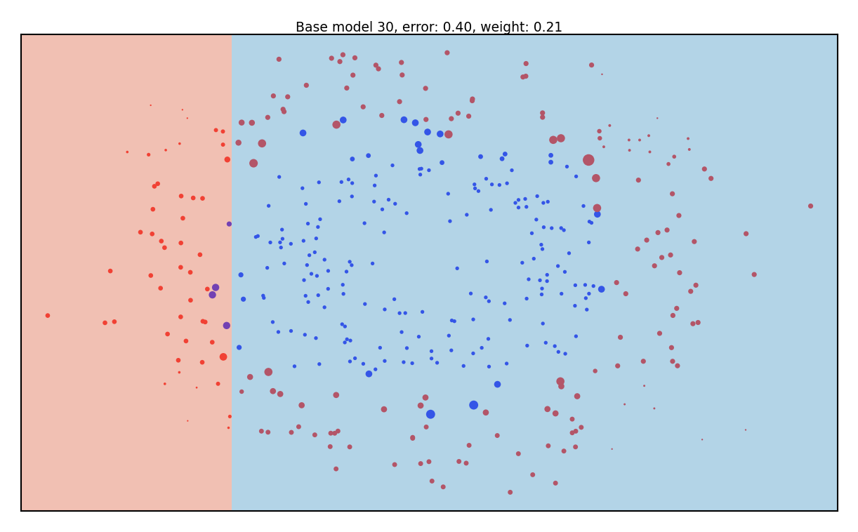
Show code cell source
if not interactive:
    fig, axes = plt.subplots(2, 2, subplot_kw={'xticks': (()), 'yticks': (())}, figsize=(11*fig_scale, 6*fig_scale))
    weight_scale = 0.5
    for iteration, ax in zip([1, 5, 37, 59],axes.flatten()):
        current_ax = ax
        plot_adaboost(iteration)
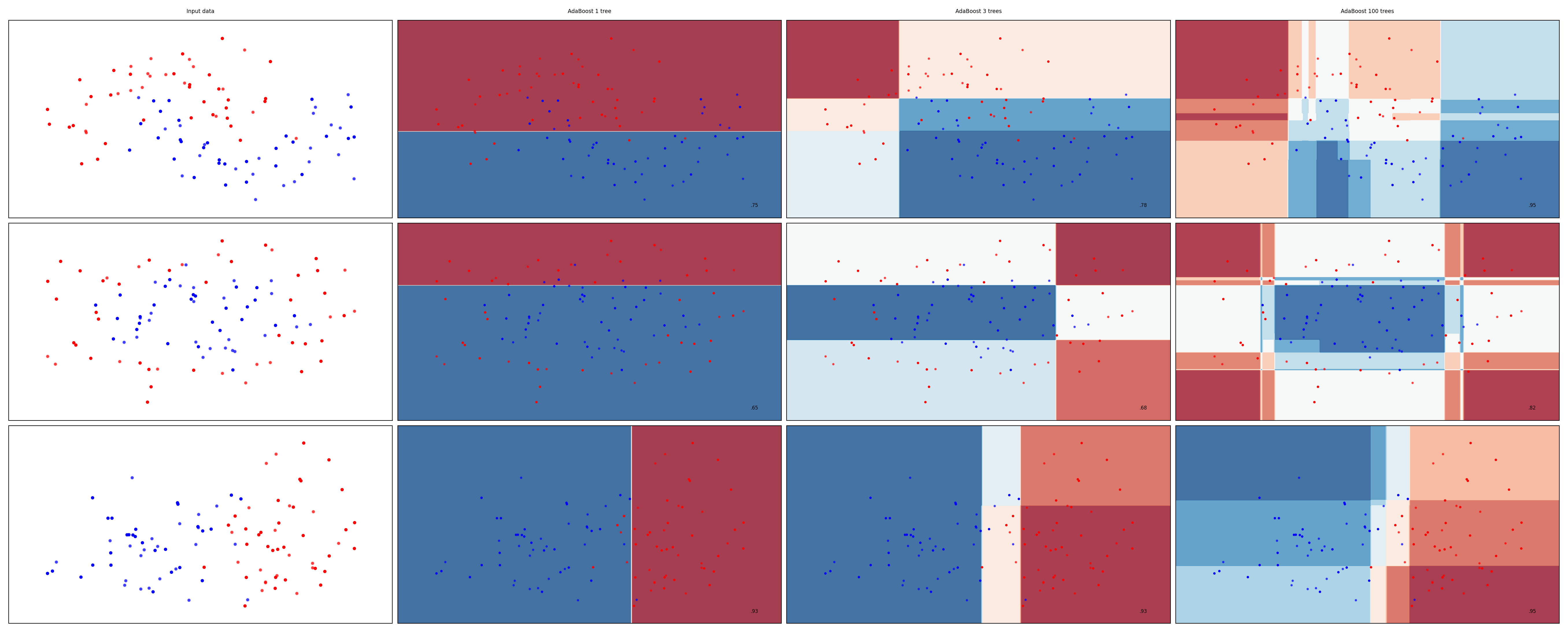
Examples#
Show code cell source
from sklearn.ensemble import AdaBoostClassifier
names = ["AdaBoost 1 tree", "AdaBoost 3 trees", "AdaBoost 100 trees"]

classifiers = [
    AdaBoostClassifier(n_estimators=1, random_state=0, learning_rate=0.5),
    AdaBoostClassifier(n_estimators=3, random_state=0, learning_rate=0.5),
    AdaBoostClassifier(n_estimators=100, random_state=0, learning_rate=0.5)
    ]

mglearn.plots.plot_classifiers(names, classifiers, figuresize=(20*fig_scale,8*fig_scale))
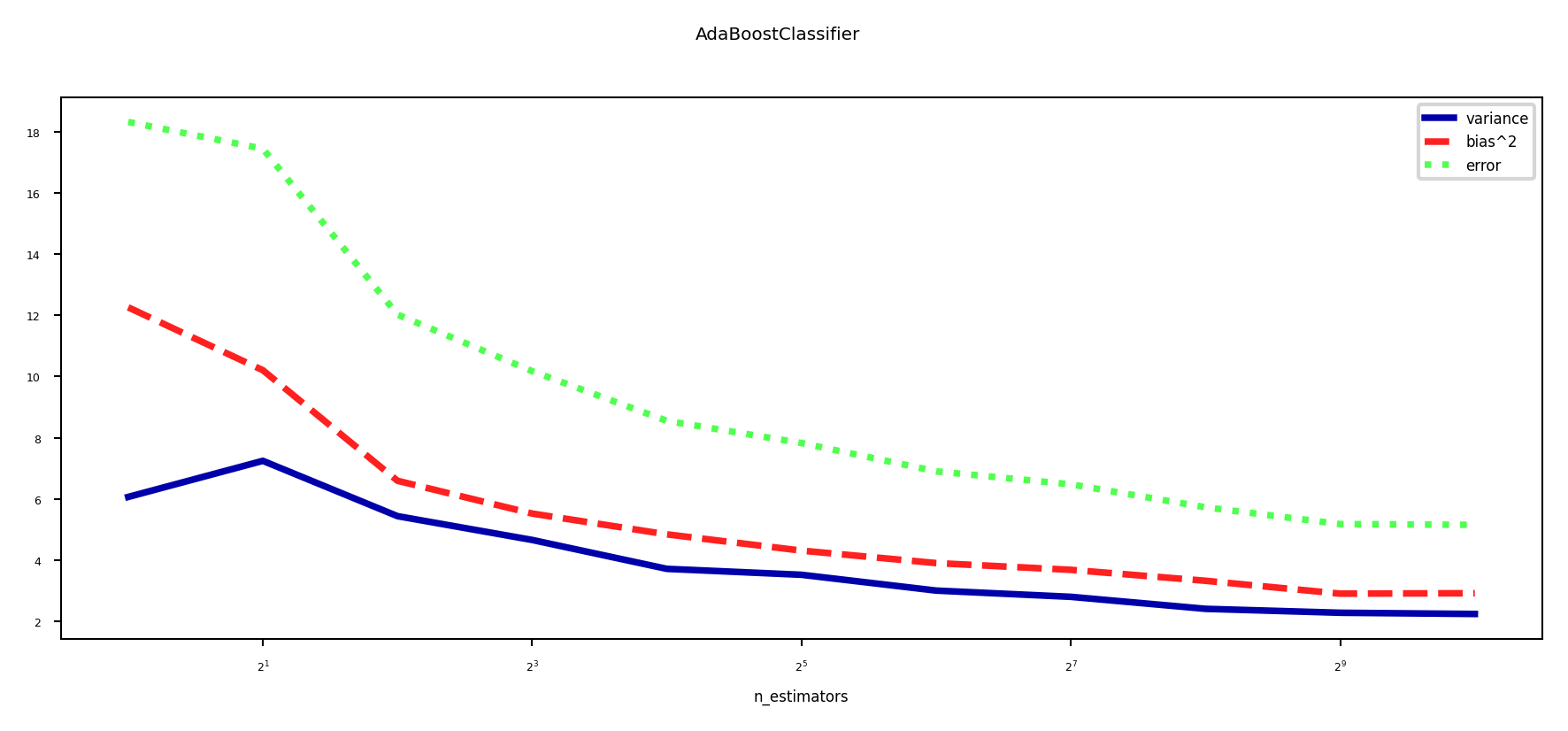
Bias-Variance analysis#
AdaBoost reduces bias (and a little variance)
Boosting is a bias reduction technique
Boosting too much will eventually increase variance
Show code cell source
plot_bias_variance_rf(AdaBoostClassifier, cancer.data, cancer.target, warm_start=False)
Gradient Boosting#
Ensemble of models, each fixing the remaining mistakes of the previous ones
Each iteration, the task is to predict the residual error of the ensemble
Additive model: Predictions at iteration \(I\) are sum of base model predictions
Learning rate (or shrinkage ) \(\eta\): small updates work better (reduces variance) $\(f_I(\mathbf{x}) = g_0(\mathbf{x}) + \sum_{i=1}^I \eta \cdot g_i(\mathbf{x}) = f_{I-1}(\mathbf{x}) + \eta \cdot g_I(\mathbf{x})\)$
The pseudo-residuals \(r_i\) are computed according to differentiable loss function
E.g. least squares loss for regression and log loss for classification
Gradient descent: predictions get updated step by step until convergence $\(g_i(\mathbf{x}) \approx r_{i} = - \frac{\partial \mathcal{L}(y_i,f_{i-1}(x_i))}{\partial f_{i-1}(x_i)}\)$
Base models \(g_i\) should be low variance, but flexible enough to predict residuals accurately
E.g. decision trees of depth 2-5
Gradient Boosting Trees (Regression)#
Base models are regression trees, loss function is square loss: \(\mathcal{L} = \frac{1}{2}(y_i - \hat{y}_i)^2\)
The pseudo-residuals are simply the prediction errors for every sample: $\(r_i = -\frac{\partial \mathcal{L}}{\partial \hat{y}} = -2 * \frac{1}{2}(y_i - \hat{y}_i) * (-1) = y_i - \hat{y}_i\)$
Initial model \(g_0\) simply predicts the mean of \(y\)
For iteration \(m=1..M\):
For all samples i=1..n, compute pseudo-residuals \(r_i = y_i - \hat{y}_i\)
Fit a new regression tree model \(g_m(\mathbf{x})\) to \(r_{i}\)
In \(g_m(\mathbf{x})\), each leaf predicts the mean of all its values
Update ensemble predictions \(\hat{y} = g_0(\mathbf{x}) + \sum_{m=1}^M \eta \cdot g_m(\mathbf{x})\)
Early stopping (optional): stop when performance on validation set does not improve for \(nr\) iterations
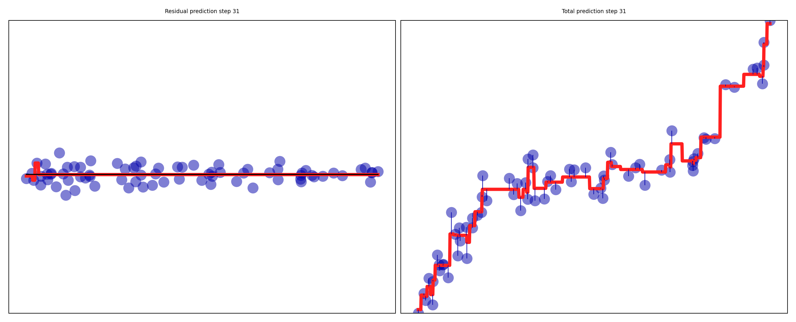
Gradient Boosting Regression in action#
Residuals quickly drop to (near) zero
Show code cell source
# Example adapted from Andreas Mueller
from sklearn.ensemble import GradientBoostingRegressor

# Make some toy data
def make_poly(n_samples=100):
    rnd = np.random.RandomState(42)
    x = rnd.uniform(-3, 3, size=n_samples)
    y_no_noise = (x) ** 3
    y = (y_no_noise + rnd.normal(scale=3, size=len(x))) / 2
    return x.reshape(-1, 1), y
Xp, yp = make_poly()

# Train gradient booster and get predictions
Xp_train, Xp_test, yp_train, yp_test = train_test_split(Xp, yp, random_state=0)
gbrt = GradientBoostingRegressor(max_depth=2, n_estimators=61, learning_rate=.3, random_state=0).fit(Xp_train, yp_train)
gbrt.score(Xp_test, yp_test)

line = np.linspace(Xp.min(), Xp.max(), 1000)
preds = list(gbrt.staged_predict(line[:, np.newaxis]))
preds_train = [np.zeros(len(yp_train))] + list(gbrt.staged_predict(Xp_train))

# Plot
def plot_gradient_boosting_step(step, axes):
    axes[0].plot(Xp_train[:, 0], yp_train - preds_train[step], 'o', alpha=0.5, markersize=10*fig_scale)
    axes[0].plot(line, gbrt.estimators_[step, 0].predict(line[:, np.newaxis]), linestyle='-', lw=3*fig_scale)
    axes[0].plot(line, [0]*len(line), c='k', linestyle='-', lw=1*fig_scale)
    axes[1].plot(Xp_train[:, 0], yp_train, 'o',  alpha=0.5, markersize=10*fig_scale)
    axes[1].plot(line, preds[step], linestyle='-', lw=3*fig_scale)
    axes[1].vlines(Xp_train[:, 0], yp_train, preds_train[step+1])

    axes[0].set_title("Residual prediction step {}".format(step + 1))
    axes[1].set_title("Total prediction step {}".format(step + 1))
    axes[0].set_ylim(yp.min(), yp.max())
    axes[1].set_ylim(yp.min(), yp.max())
    plt.tight_layout();

@interact
def plot_gradient_boosting(step = (0, 60, 1)):
    fig, axes = plt.subplots(1, 2, subplot_kw={'xticks': (()), 'yticks': (())}, figsize=(10*fig_scale, 4*fig_scale))
    plot_gradient_boosting_step(step, axes)
Show code cell source
if not interactive:
    fig, all_axes = plt.subplots(3, 2, subplot_kw={'xticks': (()), 'yticks': (())}, figsize=(10*fig_scale, 5*fig_scale))
    for i, s in enumerate([0,3,9]):
        axes = all_axes[i,:]
        plot_gradient_boosting_step(s, axes)
GradientBoosting Algorithm (Classification)#
Base models are regression trees, predict probability of positive class \(p\)
For multi-class problems, train one tree per class
Use (binary) log loss, with true class \(y_i \in {0,1}\): \(\mathcal{L_{log}} = - \sum_{i=1}^{N} \big[ y_i log(p_i) + (1-y_i) log(1-p_i) \big] \)
The pseudo-residuals are simply the difference between true class and predicted \(p\): $\(\frac{\partial \mathcal{L}}{\partial \hat{y}} = \frac{\partial \mathcal{L}}{\partial log(p_i)} = y_i - p_i\)$
Initial model \(g_0\) predicts \(p = log(\frac{\#positives}{\#negatives})\)
For iteration \(m=1..M\):
For all samples i=1..n, compute pseudo-residuals \(r_i = y_i - p_i\)
Fit a new regression tree model \(g_m(\mathbf{x})\) to \(r_{i}\)
In \(g_m(\mathbf{x})\), each leaf predicts \(\frac{\sum_{i} r_i}{\sum_{i} p_i(1-p_i)}\)
Update ensemble predictions \(\hat{y} = g_0(\mathbf{x}) + \sum_{m=1}^M \eta \cdot g_m(\mathbf{x})\)
Early stopping (optional): stop when performance on validation set does not improve for \(nr\) iterations
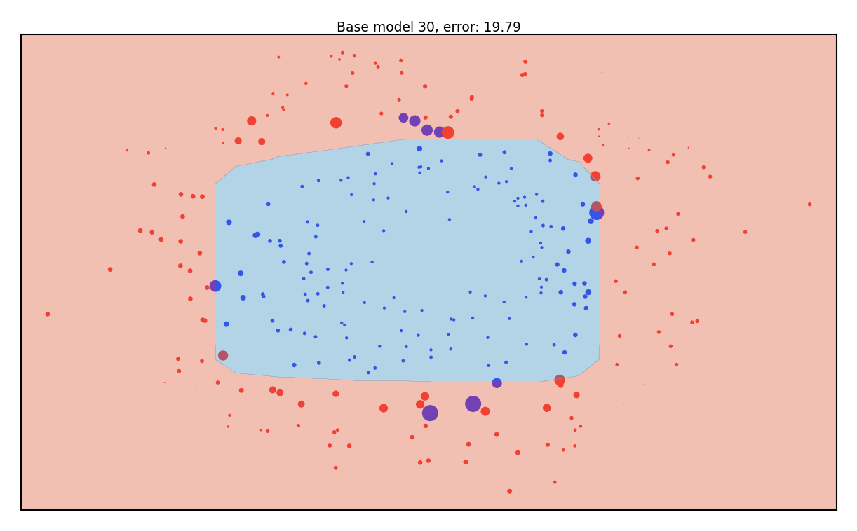
Gradient Boosting Classification in action#
Size of the samples represents the residual weights: most quickly drop to (near) zero
Show code cell source
from sklearn.ensemble import GradientBoostingClassifier

Xa_train, Xa_test, ya_train, ya_test = train_test_split(Xa, ya, random_state=0)
gbct = GradientBoostingClassifier(max_depth=2, n_estimators=60, learning_rate=.3, random_state=0).fit(Xa_train, ya_train)
gbct.score(Xa_test, ya_test)
preds_train_cl = [np.zeros(len(ya_train))] + list(gbct.staged_predict_proba(Xa_train))
current_gb_ax = None
weight_scale = 1

def plot_gb_decision_boundary(gbmodel, step, X, y, N = 10, scatter_weights = np.ones(len(y)) , ax = None, title = None ):
    '''Utility function to plot decision boundary and scatter plot of data'''
    x_min, x_max = X[:, 0].min() - .1, X[:, 0].max() + .1
    y_min, y_max = X[:, 1].min() - .1, X[:, 1].max() + .1

    # Get current axis and plot
    if ax is None:
        ax = plt.gca()
    cm_bright = ListedColormap(['#FF0000', '#0000FF'])
    ax.scatter(X[:,0],X[:,1], c = y, cmap = cm_bright, s = scatter_weights * 40, edgecolors='none')
    ax.set_xticks(())
    ax.set_yticks(())
    if title:
        ax.set_title(title, pad='0.5')

    # Plot classifier background
    if gbmodel is not None:
        xx, yy = np.meshgrid( np.linspace(x_min, x_max, N), np.linspace(y_min, y_max, N))
        zz = np.array( [list(gbmodel.staged_predict_proba(np.array([xi,yi]).reshape(1,-1)))[step][:,1] for  xi, yi in zip(np.ravel(xx), np.ravel(yy)) ] )
        Z = zz.reshape(xx.shape)
        ax.contourf(xx, yy, Z, 2, cmap='RdBu', alpha=.5, levels=[0,0.5,1])


@interact
def plot_gboost(iteration=(1,60,1)):
    pseudo_residuals = np.abs(ya_train - preds_train_cl[iteration][:,1])
    title = "Base model {}, error: {:.2f}".format(iteration,np.sum(pseudo_residuals))
    plot_gb_decision_boundary(gbct, (iteration-1), Xa_train, ya_train, N = 20, scatter_weights =pseudo_residuals * weight_scale, ax=current_gb_ax, title=title )
Show code cell source
if not interactive:
    fig, axes = plt.subplots(2, 2, subplot_kw={'xticks': (()), 'yticks': (())}, figsize=(10*fig_scale, 6*fig_scale))
    weight_scale = 0.3
    for iteration, ax in zip([1, 5, 17, 59],axes.flatten()):
        current_gb_ax = ax
        plot_gboost(iteration)
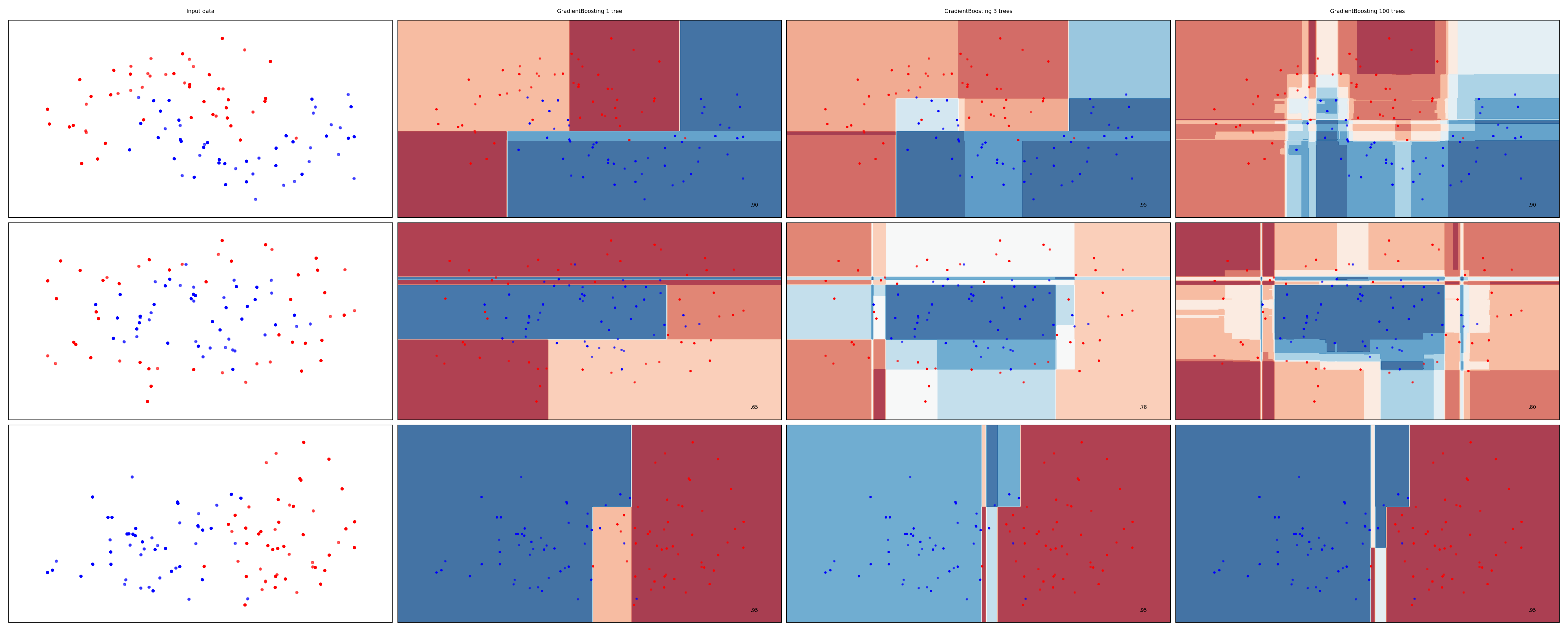
Examples#
Show code cell source
names = ["GradientBoosting 1 tree", "GradientBoosting 3 trees", "GradientBoosting 100 trees"]

classifiers = [
    GradientBoostingClassifier(n_estimators=1, random_state=0, learning_rate=0.5),
    GradientBoostingClassifier(n_estimators=3, random_state=0, learning_rate=0.5),
    GradientBoostingClassifier(n_estimators=100, random_state=0, learning_rate=0.5)
    ]

mglearn.plots.plot_classifiers(names, classifiers, figuresize=(20*fig_scale,8*fig_scale))
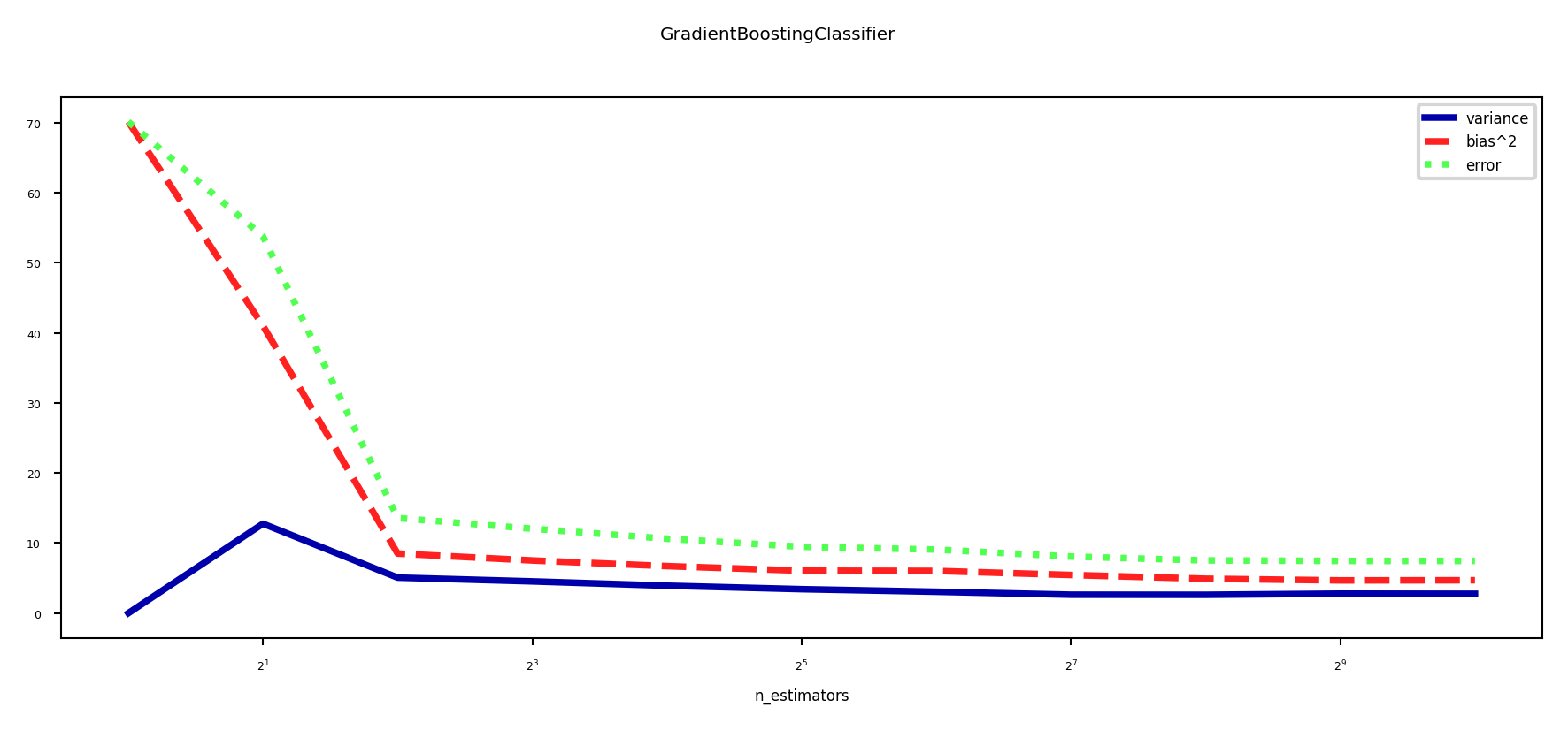
Bias-variance analysis#
Gradient Boosting is very effective at reducing bias error
Boosting too much will eventually increase variance
Show code cell source
# Note: I tried if HistGradientBoostingClassifier is faster. It's not.
# We're training many small models here and the thread spawning likely causes too much overhead
plot_bias_variance_rf(GradientBoostingClassifier, cancer.data, cancer.target, warm_start=True)
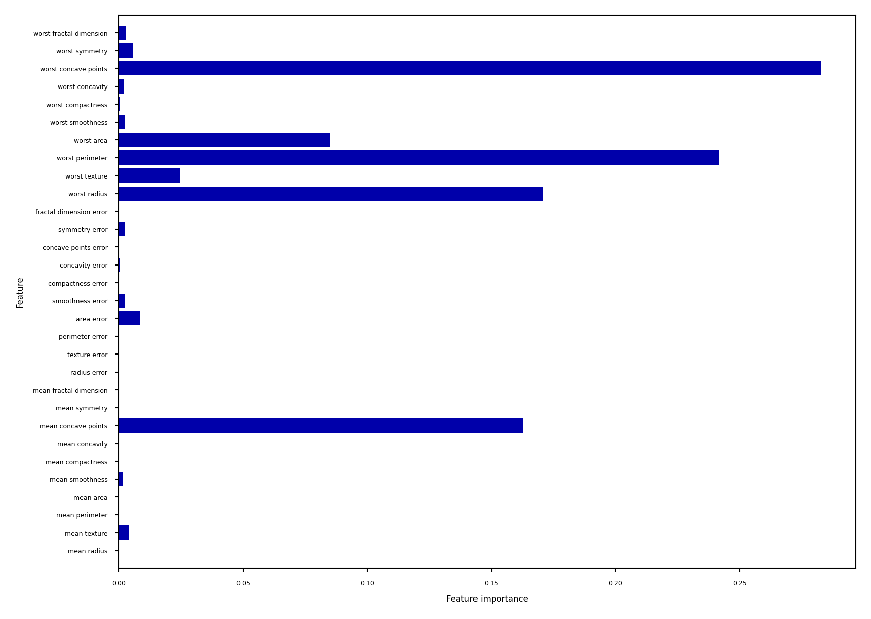
Feature importance#
Gradient Boosting also provide feature importances, based on many trees
Compared to RandomForests, the trees are smaller, hence more features have zero importance
Show code cell source
gbrt = GradientBoostingClassifier(random_state=0, max_depth=1)
gbrt.fit(Xc_train, yc_train)
plot_feature_importances_cancer(gbrt)
Gradient Boosting: strengths and weaknesses#
Among the most powerful and widely used models
Work well on heterogeneous features and different scales
Typically better than random forests, but requires more tuning, longer training
Does not work well on high-dimensional sparse data
Main hyperparameters:
n_estimators: Higher is better, but will start to overfitlearning_rate: Lower rates mean more trees are needed to get more complex modelsSet
n_estimatorsas high as possible, then tunelearning_rateOr, choose a
learning_rateand use early stopping to avoid overfitting
max_depth: typically kept low (<5), reduce when overfittingmax_features: can also be tuned, similar to random forestsn_iter_no_change: early stopping: algorithm stops if improvement is less than a certain tolerancetolfor more thann_iter_no_changeiterations.
Extreme Gradient Boosting (XGBoost)#
Faster version of gradient boosting: allows more iterations on larger datasets
Normal regression trees: split to minimize squared loss of leaf predictions
XGBoost trees only fit residuals: split so that residuals in leaf are more similar
Don’t evaluate every split point, only \(q\) quantiles per feature (binning)
\(q\) is hyperparameter (
sketch_eps, default 0.03)
For large datasets, XGBoost uses approximate quantiles
Can be parallelized (multicore) by chunking the data and combining histograms of data
For classification, the quantiles are weighted by \(p(1-p)\)
Gradient descent sped up by using the second derivative of the loss function
Strong regularization by pre-pruning the trees
Column and row are randomly subsampled when computing splits
Support for out-of-core computation (data compression in RAM, sharding,…)
XGBoost in practice#
Not part of scikit-learn, but
HistGradientBoostingClassifieris similarbinning, multicore,…
The
xgboostpython package is sklearn-compatibleInstall separately,
conda install -c conda-forge xgboostAllows learning curve plotting and warm-starting
Further reading:
LightGBM#
Another fast boosting technique
Uses gradient-based sampling
use all instances with large gradients/residuals (e.g. 10% largest)
randomly sample instances with small gradients, ignore the rest
intuition: samples with small gradients are already well-trained.
requires adapted information gain criterion
Does smarter encoding of categorical features
CatBoost#
Another fast boosting technique
Optimized for categorical variables
Uses bagged and smoothed version of target encoding
Uses symmetric trees: same split for all nodes on a given level
Can be much faster
Allows monotonicity constraints for numeric features
Model must be be a non-decreasing function of these features
Lots of tooling (e.g. GPU training)
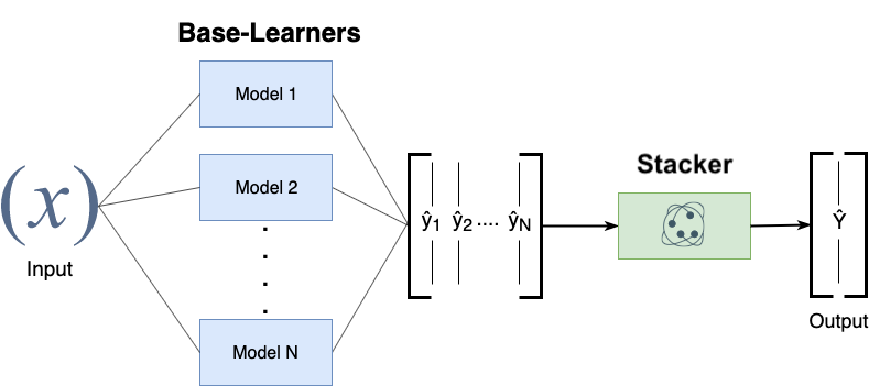
Stacking#
Choose \(M\) different base-models, generate predictions
Stacker (meta-model) learns mapping between predictions and correct label
Can also be repeated: multi-level stacking
Popular stackers: linear models (fast) and gradient boosting (accurate)
Cascade stacking: adds base-model predictions as extra features
Models need to be sufficiently different, be experts at different parts of the data
Can be very accurate, but also very slow to predict
Other ensembling techniques#
Hyper-ensembles: same basic model but with different hyperparameter settings
Can combine overfitted and underfitted models
Deep ensembles: ensembles of deep learning models
Bayes optimal classifier: ensemble of all possible models (largely theoretic)
Bayesian model averaging: weighted average of probabilistic models, weighted by their posterior probabilities
Cross-validation selection: does internal cross-validation to select best of \(M\) models
Any combination of different ensembling techniques
Show code cell source
%%HTML
<style>
td {font-size: 20px}
th {font-size: 20px}
.rendered_html table, .rendered_html td, .rendered_html th {
    font-size: 20px;
}
</style>
Algorithm overview#
Name |
Representation |
Loss function |
Optimization |
Regularization |
|---|---|---|---|---|
Classification trees |
Decision tree |
Entropy / Gini index |
Hunt’s algorithm |
Tree depth,… |
Regression trees |
Decision tree |
Square loss |
Hunt’s algorithm |
Tree depth,… |
RandomForest |
Ensemble of randomized trees |
Entropy / Gini / Square |
(Bagging) |
Number/depth of trees,… |
AdaBoost |
Ensemble of stumps |
Exponential loss |
Greedy search |
Number/depth of trees,… |
GradientBoostingRegression |
Ensemble of regression trees |
Square loss |
Gradient descent |
Number/depth of trees,… |
GradientBoostingClassification |
Ensemble of regression trees |
Log loss |
Gradient descent |
Number/depth of trees,… |
XGBoost, LightGBM, CatBoost |
Ensemble of XGBoost trees |
Square/log loss |
2nd order gradients |
Number/depth of trees,… |
Stacking |
Ensemble of heterogeneous models |
/ |
/ |
Number of models,… |
Summary#
Ensembles of voting classifiers improve performance
Which models to choose? Consider bias-variance tradeoffs!
Bagging / RandomForest is a variance-reduction technique
Build many high-variance (overfitting) models on random data samples
The more different the models, the better
Aggregation (soft voting) over many models reduces variance
Diminishing returns, over-smoothing may increase bias error
Parallellizes easily, doesn’t require much tuning
Boosting is a bias-reduction technique
Build low-variance models that correct each other’s mistakes
By reweighting misclassified samples: AdaBoost
By predicting the residual error: Gradient Boosting
Additive models: predictions are sum of base-model predictions
Can drive the error to zero, but risk overfitting
Doesn’t parallelize easily. Slower to train, much faster to predict.
XGBoost,LightGBM,… are fast and offer some parallellization
Stacking: learn how to combine base-model predictions
Base-models still have to be sufficiently different