
Kernel Trick#
Making linear models non-linear
Mahmood Amintoosi, Spring 2025
Computer Science Dept, Ferdowsi University of Mashhad
I should mention that the original material of this course was from Open Machine Learning Course, by Joaquin Vanschoren and others.
Note: Kernel trick, which is also known as kernel method or kernel machines are a class of algorithms for pattern analysis, where involve using linear classifiers to solve nonlinear problems. These methods are different from kernelization, that is a technique for designing efficient algorithms that achieve their efficiency by a preprocessing stage in which inputs to the algorithm are replaced by a smaller input, called a “kernel”.
Show code cell source
# Auto-setup when running on Google Colab
import os
if 'google.colab' in str(get_ipython()) and not os.path.exists('/content/machine-learning'):
    !git clone -q https://github.com/fum-cs/machine-learning.git /content/machine-learning
    !pip --quiet install -r /content/machine-learning/requirements_colab.txt
    %cd machine-learning/notebooks

# Global imports and settings
%matplotlib inline
from preamble import *
interactive = True # Set to True for interactive plots
if interactive:
    fig_scale = 0.5
    plt.rcParams.update(print_config)
else: # For printing
    fig_scale = 1.3
    plt.rcParams.update(print_config)
Feature Maps#
Linear models: \(\hat{y} = \mathbf{w}\mathbf{x} + w_0 = \sum_{i=1}^{p} w_i x_i + w_0 = w_0 + w_1 x_1 + ... + w_p x_p \)
When we cannot fit the data well, we can add non-linear transformations of the features
Feature map (or basis expansion ) \(\phi\) : \( X \rightarrow \mathbb{R}^d \)
E.g. Polynomial feature map: all polynomials up to degree \(d\) and all products
Example with \(p=1, d=3\) :
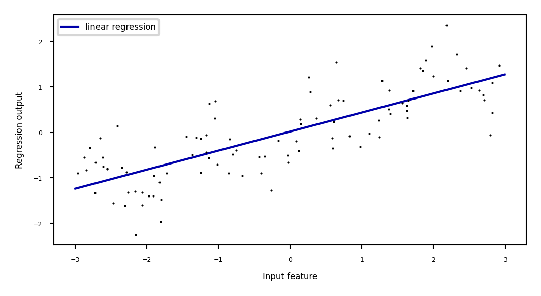
Ridge regression example#
Show code cell source
from sklearn.linear_model import Ridge

X, y = mglearn.datasets.make_wave(n_samples=100)
line = np.linspace(-3, 3, 1000, endpoint=False).reshape(-1, 1)
reg = Ridge().fit(X, y)
print("Weights:",reg.coef_)
fig = plt.figure(figsize=(8*fig_scale,4*fig_scale))
plt.plot(line, reg.predict(line), label="linear regression", lw=2*fig_scale)

plt.plot(X[:, 0], y, 'o', c='k')
plt.ylabel("Regression output")
plt.xlabel("Input feature")
plt.legend(loc="best")
Weights: [0.418]
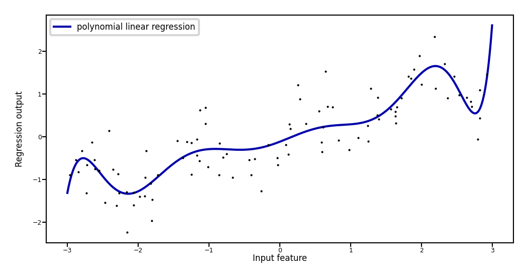
Add all polynomials \(x^d\) up to degree 10 and fit again:
e.g. use sklearn
PolynomialFeatures
Show code cell source
from sklearn.preprocessing import PolynomialFeatures

# include polynomials up to x ** 10:
# the default "include_bias=True" adds a feature that's constantly 1
poly = PolynomialFeatures(degree=10, include_bias=False)
poly.fit(X)
X_poly = poly.transform(X)
styles = [dict(selector="td", props=[("font-size", "150%")]),dict(selector="th", props=[("font-size", "150%")])]
pd.DataFrame(X_poly, columns=poly.get_feature_names_out()).head().style.set_table_styles(styles)
| x0 | x0^2 | x0^3 | x0^4 | x0^5 | x0^6 | x0^7 | x0^8 | x0^9 | x0^10 | |
|---|---|---|---|---|---|---|---|---|---|---|
| 0 | -0.752759 | 0.566647 | -0.426548 | 0.321088 | -0.241702 | 0.181944 | -0.136960 | 0.103098 | -0.077608 | 0.058420 |
| 1 | 2.704286 | 7.313162 | 19.776880 | 53.482337 | 144.631526 | 391.124988 | 1057.713767 | 2860.360362 | 7735.232021 | 20918.278410 |
| 2 | 1.391964 | 1.937563 | 2.697017 | 3.754150 | 5.225640 | 7.273901 | 10.125005 | 14.093639 | 19.617834 | 27.307312 |
| 3 | 0.591951 | 0.350406 | 0.207423 | 0.122784 | 0.072682 | 0.043024 | 0.025468 | 0.015076 | 0.008924 | 0.005283 |
| 4 | -2.063888 | 4.259634 | -8.791409 | 18.144485 | -37.448187 | 77.288869 | -159.515582 | 329.222321 | -679.478050 | 1402.366700 |
Show code cell source
reg = Ridge().fit(X_poly, y)
print("Weights:",reg.coef_)
line_poly = poly.transform(line)
fig = plt.figure(figsize=(8*fig_scale,4*fig_scale))
plt.plot(line, reg.predict(line_poly), label='polynomial linear regression', lw=2*fig_scale)
plt.plot(X[:, 0], y, 'o', c='k')
plt.ylabel("Regression output")
plt.xlabel("Input feature", labelpad=0.1)
plt.tick_params(axis='both', pad=0.1)
plt.legend(loc="best");
Weights: [ 0.643 0.297 -0.69 -0.264 0.41 0.096 -0.076 -0.014 0.004 0.001]
How expensive is this?#
You may need MANY dimensions to fit the data
Memory and computational cost
More weights to learn, more likely overfitting
Ridge has a closed-form solution which we can compute with linear algebra: $\(w^{*} = (X^{T}X + \alpha I)^{-1} X^T Y\)$
Since X has \(n\) rows (examples), and \(d\) columns (features), \(X^{T}X\) has dimensionality \(d \times d\)
Hence Ridge is quadratic in the number of features, \(\mathcal{O}(d^2n)\)
After the feature map \(\Phi\), we get $\(w^{*} = (\Phi(X)^{T}\Phi(X) + \alpha I)^{-1} \Phi(X)^T Y\)$
Since \(\Phi\) increases \(d\) a lot, \(\Phi(X)^{T}\Phi(X)\) becomes huge
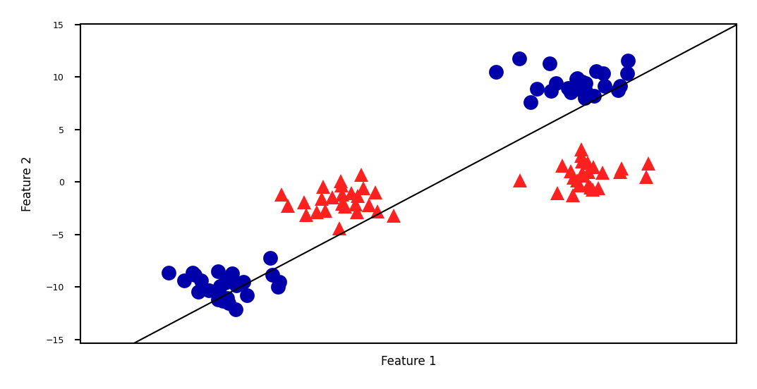
Linear SVM example (classification)#
Show code cell source
from sklearn.datasets import make_blobs
from sklearn.svm import LinearSVC
X, y = make_blobs(centers=4, random_state=8)
y = y % 2
linear_svm = LinearSVC().fit(X, y)

fig = plt.figure(figsize=(8*fig_scale,4*fig_scale))
mglearn.plots.plot_2d_separator(linear_svm, X)
mglearn.discrete_scatter(X[:, 0], X[:, 1], y, s=10*fig_scale)
plt.xlabel("Feature 1")
plt.ylabel("Feature 2");
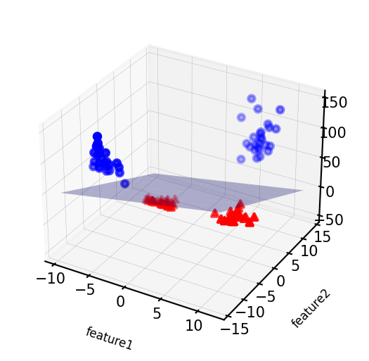
We can add a new feature by taking the squares of feature1 values
Show code cell source
# add the squared first feature
X_new = np.hstack([X, X[:, 1:] ** 2])

# visualize in 3D
fig = plt.figure(figsize=(8*fig_scale,4*fig_scale))
ax = fig.add_subplot(111, projection='3d')

# plot first all the points with y==0, then all with y == 1
mask = y == 0
ax.scatter(X_new[mask, 0], X_new[mask, 1], X_new[mask, 2], c='b',
           cmap=mglearn.cm2, s=10*fig_scale)
ax.scatter(X_new[~mask, 0], X_new[~mask, 1], X_new[~mask, 2], c='r', marker='^',
           cmap=mglearn.cm2, s=10*fig_scale)
ax.set_xlabel("feature1", labelpad=-9)
ax.set_ylabel("feature2", labelpad=-9)
ax.set_zlabel("feature2 ** 2", labelpad=-9);
ax.tick_params(axis='both', width=0, labelsize=5*fig_scale, pad=-3)
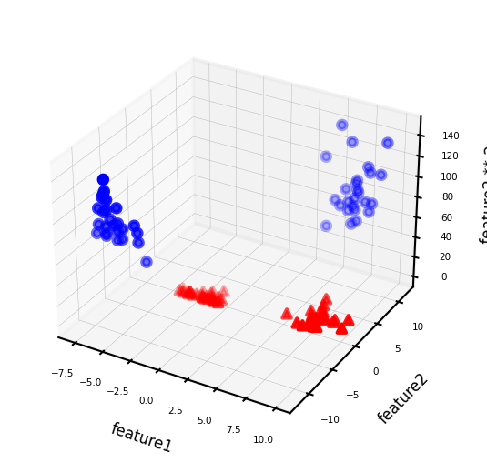
Now we can fit a linear model
Show code cell source
linear_svm_3d = LinearSVC().fit(X_new, y)
coef, intercept = linear_svm_3d.coef_.ravel(), linear_svm_3d.intercept_

# show linear decision boundary
fig = plt.figure(figsize=(8*fig_scale,4*fig_scale))
ax = fig.add_subplot(111, projection='3d')
xx = np.linspace(X_new[:, 0].min() - 2, X_new[:, 0].max() + 2, 50)
yy = np.linspace(X_new[:, 1].min() - 2, X_new[:, 1].max() + 2, 50)

XX, YY = np.meshgrid(xx, yy)
ZZ = (coef[0] * XX + coef[1] * YY + intercept) / -coef[2]
ax.plot_surface(XX, YY, ZZ, rstride=8, cstride=8, alpha=0.3)
ax.scatter(X_new[mask, 0], X_new[mask, 1], X_new[mask, 2], c='b',
           cmap=mglearn.cm2, s=10*fig_scale)
ax.scatter(X_new[~mask, 0], X_new[~mask, 1], X_new[~mask, 2], c='r', marker='^',
           cmap=mglearn.cm2, s=10*fig_scale)

ax.set_xlabel("feature1", labelpad=-9)
ax.set_ylabel("feature2", labelpad=-9)
ax.set_zlabel("feature2 ** 2", labelpad=-9);
ax.tick_params(axis='both', width=0, labelsize=10*fig_scale, pad=-6)
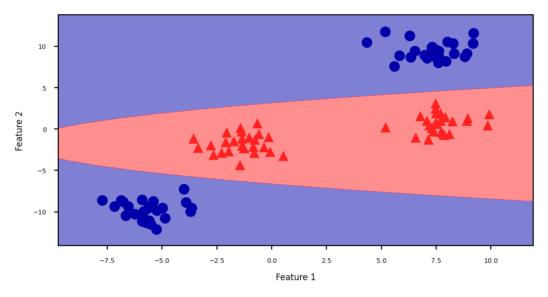
As a function of the original features, the decision boundary is now a polynomial as well $\(y = w_0 + w_1 x_1 + w_2 x_2 + w_3 x_2^2 > 0\)$
Show code cell source
ZZ = YY ** 2
dec = linear_svm_3d.decision_function(np.c_[XX.ravel(), YY.ravel(), ZZ.ravel()])
figure = plt.figure(figsize=(8*fig_scale,4*fig_scale))
plt.contourf(XX, YY, dec.reshape(XX.shape), levels=[dec.min(), 0, dec.max()],
             cmap=mglearn.cm2, alpha=0.5)
mglearn.discrete_scatter(X[:, 0], X[:, 1], y, s=10*fig_scale)
plt.xlabel("Feature 1")
plt.ylabel("Feature 2");
The kernel trick#
Computations in explicit, high-dimensional feature maps are expensive
For some feature maps, we can, however, compute distances between points cheaply
Without explicitly constructing the high-dimensional space at all
Example: quadratic feature map for \(\mathbf{x} = (x_1,..., x_p )\):
A kernel function exists for this feature map to compute dot products
Skip computation of \(\Phi(x_i)\) and \(\Phi(x_j)\) and compute \(k(x_i,x_j)\) directly
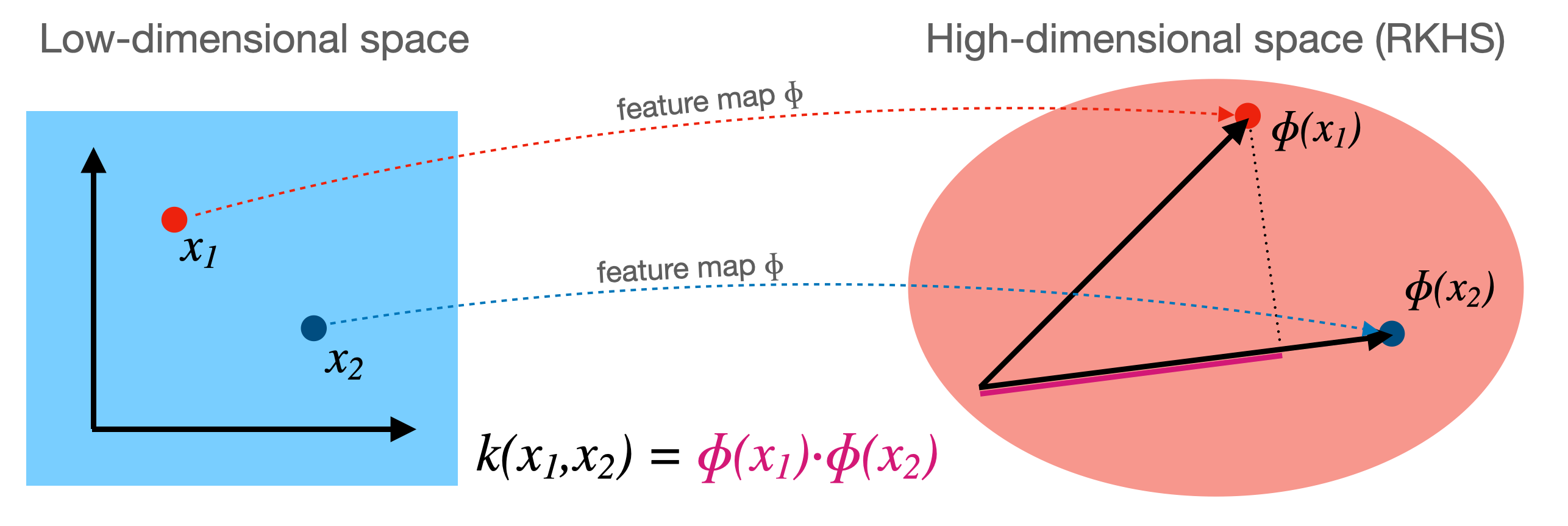
Kernel Method#
Kernel \(k\) corresponding to a feature map \(\Phi\): \( k(\mathbf{x_i},\mathbf{x_j}) = \Phi(\mathbf{x_i}) \cdot \Phi(\mathbf{x_j})\)
Computes dot product between \(x_i,x_j\) in a high-dimensional space \(\mathcal{H}\)
Kernels are sometimes called generalized dot products
\(\mathcal{H}\) is called the reproducing kernel Hilbert space (RKHS)
The dot product is a measure of the similarity between \(x_i,x_j\)
Hence, a kernel can be seen as a similarity measure for high-dimensional spaces
If we have a loss function based on dot products \(\mathbf{x_i}\cdot\mathbf{x_j}\) it can be kernelized
Simply replace the dot products with \(k(\mathbf{x_i},\mathbf{x_j})\)
Chapter 5 of Zaki book#
Kernel K-Means#
Other examples#
For Kernel PCA, see section 7.3 of Zaki Book
For Kernel SMV and Kernel Regression see Appendix A
Summary#
Feature maps \(\Phi(x)\) transform features to create a higher-dimensional space
Allows learning non-linear functions or boundaries, but very expensive/slow
For some \(\Phi(x)\), we can compute dot products without constructing this space
Kernel trick: \(k(\mathbf{x_i},\mathbf{x_j}) = \Phi(\mathbf{x_i}) \cdot \Phi(\mathbf{x_j})\)
Kernel \(k\) (generalized dot product) is a measure of similarity between \(\mathbf{x_i}\) and \(\mathbf{x_j}\)
There are many such kernels
Polynomial kernel: \(k_{poly}(\mathbf{x_1},\mathbf{x_2}) = (\gamma (\mathbf{x_1} \cdot \mathbf{x_2}) + c_0)^d\)
RBF (Gaussian) kernel: \(k_{RBF}(\mathbf{x_1},\mathbf{x_2}) = exp(-\gamma ||\mathbf{x_1} - \mathbf{x_2}||^2)\)
A kernel matrix can be precomputed using any similarity measure (e.g. for text, graphs,…)
Any loss function where inputs appear only as dot products can be kernelized
E.g. Linear SVMs: simply replace the dot product with a kernel of choice
The Representer theorem states which other loss functions can also be kernelized and how
Ridge regression, Logistic regression, Perceptrons,…