Maximum Likelihood Estimation (MLE)

Course: Statistical Machine Learning

Reference: Duda, R. O., Hart, P. E., & Stork, D. G. (2000). Pattern Classification (2nd ed.). Wiley-Interscience.

Topic: Parametric Density Estimation

1. Introduction¶

In statistical pattern classification, a common assumption is that the data is generated by an underlying probability distribution with unknown parameters. For example, we may assume the features $x$ follow a Gaussian (Normal) distribution. To make optimal decisions (e.g., classification using Bayes decision theory), we must estimate the parameters of these distributions from a training dataset.

Maximum Likelihood Estimation (MLE) is a standard parametric method used to estimate the unknown parameters $\theta$ of a probability density function $p(x|\theta)$ given a dataset $\mathcal{D}$ . The principle is to select the parameter values that make the observed data most probable.

2. The Likelihood Function¶

The likelihood function, denoted as $L(\theta|\mathcal{D})$ , represents the probability of observing the specific dataset $\mathcal{D}$ as a function of the parameters $\theta$ .

Key Distinction:
It is crucial to distinguish between the probability density function $p(x|\theta)$ and the likelihood function $L(\theta|\mathcal{D})$ :

$p(x|\theta)$ : Describes the distribution of the data $x$ for fixed parameters $\theta$ .
$L(\theta|\mathcal{D})$ : Describes the probability of the dataset $\mathcal{D}$ for fixed observed data, viewed as a function of $\theta$ .

The likelihood function lives in a different space than the probability density function. As noted in Duda & Hart, the functional form of the likelihood is not necessarily the same as the functional form of the density.

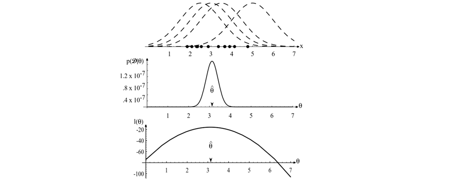
Figure 3.1: The top graph shows several training points in one dimension, known or assumed to be drawn from a Gaussian of a particular variance, but unknown mean. Four of the infinite number of candidate source distributions are shown in dashed lines. The middle figures shows the likelihood $p(\mathcal{D}|\theta)$ as a function of the mean. If we had a very large number of training points, this likelihood would be very narrow. The value that maximizes the likelihood is marked $\hat{\theta}$ ; it also maximizes the logarithm of the likelihood — i.e., the log-likelihood $l(\theta)$ , shown at the bottom. Note especially that the likelihood lies in a different space from $p(x|\hat{\theta})$ , and the two can have different functional forms.

3. Mathematical Derivation: Univariate Gaussian¶

We begin with the simplest case: estimating the parameters of a univariate Gaussian distribution. This serves as the foundation for understanding the multivariate case used in pattern classification.

3.1 Problem Definition¶

Let $\mathcal{D} = \{x_1, x_2, \dots, x_n\}$ be a dataset consisting of $n$ independent and identically distributed (i.i.d.) samples. We assume each sample is drawn from a univariate Gaussian distribution:

p(x | \mu, \sigma^2) = \frac{1}{\sqrt{2\pi\sigma^2}} \exp\left(-\frac{(x - \mu)^2}{2\sigma^2}\right)

(1)

where:

$\mu$ is the mean (location parameter).
$\sigma^2$ is the variance (scale parameter).

3.2 The Likelihood Function¶

The likelihood function $L(\mu, \sigma^2)$ is the joint probability density of the observed data, assuming independence:

\begin{aligned} L(\mu, \sigma^2) &= p(\mathcal{D} | \mu, \sigma^2) \\ &= \prod_{k=1}^n p(x_k | \mu, \sigma^2) \\ &= \prod_{k=1}^n \frac{1}{\sqrt{2\pi\sigma^2}} \exp\left(-\frac{(x_k - \mu)^2}{2\sigma^2}\right) \\ &= \left( \frac{1}{\sqrt{2\pi\sigma^2}} \right)^n \exp\left( -\sum_{k=1}^n \frac{(x_k - \mu)^2}{2\sigma^2} \right) \end{aligned}

(2)

3.3 The Log-Likelihood Function¶

Directly maximizing $L(\mu, \sigma^2)$ is computationally difficult due to the product of exponentials. Since the logarithm is a strictly monotonic function, maximizing the log-likelihood $\ell(\mu, \sigma^2)$ yields the same parameter estimates as maximizing the likelihood.

\begin{aligned} \ell(\mu, \sigma^2) &= \log L(\mu, \sigma^2) \\ &= \sum_{k=1}^n \log \left( \frac{1}{\sqrt{2\pi\sigma^2}} \exp\left(-\frac{(x_k - \mu)^2}{2\sigma^2}\right) \right) \\ &= \sum_{k=1}^n \left[ -\frac{1}{2} \log(2\pi) - \frac{1}{2} \log(\sigma^2) - \frac{(x_k - \mu)^2}{2\sigma^2} \right] \\ &= -\frac{n}{2} \log(2\pi) - \frac{n}{2} \log(\sigma^2) - \frac{1}{2\sigma^2} \sum_{k=1}^n (x_k - \mu)^2 \end{aligned}

(3)

3.4 Estimating the Mean ( $\mu$ )¶

To find the Maximum Likelihood Estimate (MLE) $\hat{\mu}$ , we take the partial derivative of $\ell$ with respect to $\mu$ and set it to zero:

\frac{\partial \ell}{\partial \mu} = \sum_{k=1}^n \frac{(x_k - \mu)}{\sigma^2} = \frac{1}{\sigma^2} \sum_{k=1}^n (x_k - \mu) = 0

(4)

Solving for $\mu$ :

\sum_{k=1}^n x_k - n\hat{\mu} = 0 \implies \hat{\mu} = \frac{1}{n} \sum_{k=1}^n x_k

(5)

Result: The MLE for the mean is the sample mean.

3.5 Estimating the Variance ( $\sigma^2$ )¶

To find the MLE $\hat{\sigma}^2$ , we take the partial derivative of $\ell$ with respect to $\sigma^2$ . Let $\tau = \sigma^2$ for simpler differentiation:

\frac{\partial \ell}{\partial \tau} = -\frac{n}{2\tau} + \frac{1}{2\tau^2} \sum_{k=1}^n (x_k - \mu)^2 = 0

(6)

Multiplying by $2\tau^2$ :

-n\tau + \sum_{k=1}^n (x_k - \mu)^2 = 0

(7)

Substituting $\hat{\mu}$ for $\mu$ and $\tau = \sigma^2$ :

\hat{\sigma}^2 = \frac{1}{n} \sum_{k=1}^n (x_k - \hat{\mu})^2

(8)

Result: The MLE for the variance is the sample variance (with denominator $n$ ).

4. Extension to Multivariate Gaussian¶

In Pattern Classification, features are typically vectors $\mathbf{x} \in \mathbb{R}^d$ . The univariate derivation extends naturally to the Multivariate Gaussian Distribution.

4.1 Density Function¶

p(\mathbf{x} | \boldsymbol{\mu}, \boldsymbol{\Sigma}) = \frac{1}{(2\pi)^{d/2} |\boldsymbol{\Sigma}|^{1/2}} \exp\left( -\frac{1}{2} (\mathbf{x} - \boldsymbol{\mu})^T \boldsymbol{\Sigma}^{-1} (\mathbf{x} - \boldsymbol{\mu}) \right)

(9)

4.2 MLE Estimates¶

Following the same log-likelihood maximization procedure:

Mean Vector ( $\boldsymbol{\mu}$ ):
$\hat{\boldsymbol{\mu}} = \frac{1}{n} \sum_{k=1}^n \mathbf{x}_k$
(10)
The MLE is the sample mean vector.
Covariance Matrix ( $\boldsymbol{\Sigma}$ ):
$\hat{\boldsymbol{\Sigma}} = \frac{1}{n} \sum_{k=1}^n (\mathbf{x}_k - \hat{\boldsymbol{\mu}})(\mathbf{x}_k - \hat{\boldsymbol{\mu}})^T$
(11)
The MLE is the sample covariance matrix.

5. Properties and Limitations¶

While MLE is a powerful tool, Duda & Hart highlight several important characteristics regarding these estimates, particularly in the context of classification:

Bias:
- The estimate for the mean $\hat{\mu}$ is unbiased.
- The estimate for the variance $\hat{\sigma}^2$ (and $\hat{\boldsymbol{\Sigma}}$ ) is biased. It systematically underestimates the true variance because it uses $n$ instead of $n-1$ in the denominator.
- Unbiased estimator: $s^2 = \frac{1}{n-1} \sum (x_k - \hat{\mu})^2$ . However, for large $n$ , the difference is negligible.
Consistency:
- As the number of samples $n \to \infty$ , the MLE estimates converge to the true parameter values.
Invariance:
- If $\hat{\theta}$ is the MLE of $\theta$ , then for any function $g(\theta)$ , the MLE of $g(\theta)$ is $g(\hat{\theta})$ .
Sensitivity to Outliers:
- Because MLE assumes the data follows a specific distribution (e.g., Gaussian), outliers can significantly skew the estimates of the mean and covariance, potentially degrading classification performance.

6. Connection to Bayesian Classification¶

The primary role of MLE in this course is to enable Bayesian Classification when parameters are unknown.

6.1 The “Plug-In” Approach¶

Train: For each class $\omega_i$ , use the training data $\mathcal{D}_i$ to compute MLE estimates $\hat{\boldsymbol{\mu}}_i$ and $\hat{\boldsymbol{\Sigma}}_i$ .
Construct: Form the estimated class-conditional density: $\hat{p}(\mathbf{x} | \omega_i) = \mathcal{N}(\mathbf{x} | \hat{\boldsymbol{\mu}}_i, \hat{\boldsymbol{\Sigma}}_i)$ .
Decide: Apply the Bayes Decision Rule using these estimated densities.

This is known as a Plug-In Classifier. It approximates the optimal Bayes classifier by plugging in the best estimate of the parameters.

6.2 Impact on Decision Boundaries¶

The MLE estimates dictate the geometry of the classifier:

Linear Discriminant Analysis (LDA): Assumes all classes share a common covariance $\boldsymbol{\Sigma}$ . The decision boundary becomes linear (hyperplane).
Quadratic Discriminant Analysis (QDA): Assumes classes have unique covariances $\boldsymbol{\Sigma}_i$ . The decision boundary becomes quadratic (hyper-ellipsoid).

7. Bridge to Advanced Topics¶

MLE is not limited to simple Gaussian classification. It is the foundational engine for many advanced models we will cover later:

Principal Component Analysis (PCA): Can be derived as a Maximum Likelihood problem for a Gaussian model with constraints (finding directions of maximum variance).
Gaussian Mixture Models (GMM): Extends single Gaussians to mixtures. MLE is used, but requires the EM Algorithm (Expectation-Maximization) for iterative solution.
Hidden Markov Models (HMM): Parameters (transition and emission probabilities) are estimated using MLE via the Forward-Backward Algorithm.

8. Summary¶

The Maximum Likelihood Estimation method provides a principled approach to learning parameters for probabilistic models in machine learning.

Key Takeaways:

Likelihood vs. Probability: We maximize the likelihood of the data given the parameters, not the probability of the parameters given the data.
Log-Likelihood: Transforming to the log-domain converts products to sums, simplifying optimization.
Univariate Results:
- $\hat{\mu} = \text{mean}(\mathcal{D})$
- $\hat{\sigma}^2 = \text{var}(\mathcal{D})$ (biased)
Relevance to Classification: These estimates are the building blocks for Linear Discriminant Analysis (LDA) and other Gaussian-based classifiers discussed later in the course.