Bayesian Decision Theory
Mahmood Amintoosi, Fall 2026
Computer Science Dept, Ferdowsi University of Mashhad
This page follows chapter 2 of Pattern Classification by Duda, Hart, and Stork (Duda et al. (2000)), including its figures and the fish example. The estimates that fill in the densities come from the MLE page; the geometry of the Gaussian case is worked out on the Mahalanobis distance page, and the naive assumption that makes the densities tractable is the subject of Naive Bayes.
Learning objectives. By the end you should be able to
write Bayes’ formula for a classification problem and say which factor is a prior, a likelihood, an evidence and a posterior;
define a loss matrix, the conditional risk, and show that the zero-one loss gives the minimum error rate rule;
derive the discriminant function for Gaussian classes in the three cases of Duda’s chapter — isotropic, equal, and arbitrary covariance matrices;
say what the decision boundary looks like in each case: a hyperplane orthogonal to the line between the means, a general hyperplane, or a quadric surface;
read the geometry off the eigenvalues of the covariance matrix.
Introduction
Bayesian Decision Theory is a statistical approach to pattern classification.
It quantifies tradeoffs between classification decisions using probabilities and costs.
Assumes all relevant probabilities are known.
Example: Classifying fish (sea bass vs. salmon) based on features like lightness.
Key Concepts
State of Nature (): Represents the true category (e.g., sea bass or salmon).
Prior Probability (): Probability of a category before observing any data.
Class-Conditional Probability Density (): Probability density of the observation given category .
Posterior Probability (): Probability of category after observing the features .
Bayes’ Formula
Bayes’ Theorem:
that is, posterior = likelihood × prior / evidence. The evidence () is the normalising constant, and it is often ignored in classification because it is the same for every class.
The fish example below is one-dimensional: there the observation is a single feature , the lightness of the fish, and is a curve rather than a surface.
Reading the Formula
It is the product of likelihood and prior that decides the posterior; the evidence is only a scale factor, present to make the posteriors sum to one. The likelihood is so called because, other things being equal, the class for which it is large is the more likely one.
Figures 2.1 and 2.2 show the two halves of the argument for the fish: the class-conditional densities, and the posteriors they produce with priors and .
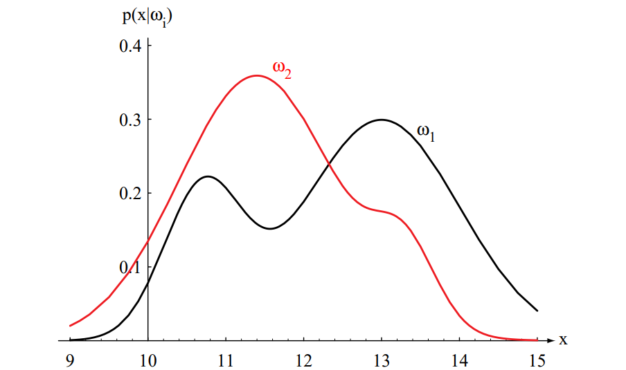
Figure 2.1: hypothetical class-conditional densities for the lightness of sea bass () and salmon (). Each curve is a density, so the area under it is 1.
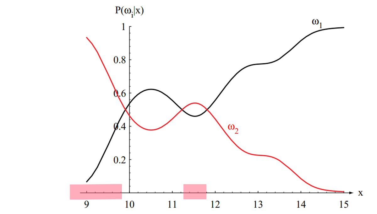
Figure 2.2: the posteriors for the densities of Figure 2.1 with and . At the posterior of is about 0.08 and that of about 0.92; at every the two posteriors sum to 1.
Risk and Decision Rules
Loss and Conditional Risk
The minimum-error rule is a special case of a more general criterion. Let be the actions available — for classification, “decide ” — and let be the loss of taking action when the true class is . The conditional risk of action for an observation is
and the Bayes decision rule selects the action of least risk:
The zero-one loss sets when and 1 otherwise, that is, it prices every error the same. Its conditional risk is the probability of being wrong,
so minimising the risk is the same as maximising the posterior. Unequal losses — a missed disease costing more than a false alarm — simply move the decision threshold; they do not change the machinery.
Minimum Error Rate Classification
Decide if , otherwise decide .
Equivalently, since the evidence is common to both classes, decide if
The probability of error for a given observation is
Special Cases
Two cases show which factor drives the decision.
If , the observation is equally likely under both classes and tells us nothing; the decision rests entirely on the priors.
If , the classes are equally probable a priori and the decision rests entirely on the likelihoods.
In general both matter, and the rule combines them; that combination is what minimises the probability of error.
More Than Two Classes
With classes the same rule applies unchanged: assign to the class that maximises the posterior, which — as shown above — is the action of least risk under the zero-one loss:
For each class we compute one posterior, and the regions where class wins are separated by the surfaces .
Discriminant Functions
A discriminant function is any function whose value is largest for the class we want to choose; the classifier computes one per class and picks the maximum.
For minimum error rate the obvious choice is the posterior itself,
and because the evidence is a common positive factor we may use the numerator,
or its logarithm, which turns the product into a sum and the exponential of a Gaussian into a quadratic form:
Any monotone function of a discriminant is a discriminant, and any positive multiple or additive constant may be dropped: the classification is unchanged. That freedom is what makes the Gaussian case tractable below.
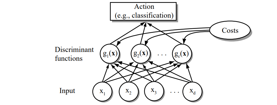
Figure 2.5: the structure of a general statistical classifier — inputs, discriminant functions, and a maximum selector. The arrows show the flow of information.
The Normal Density
Univariate Case
The univariate normal density is
with the expected value of (an average over the feature space)
and the variance
The univariate normal is completely specified by and ; we write . Samples cluster about the mean with a spread set by the standard deviation (Figure 2.7).
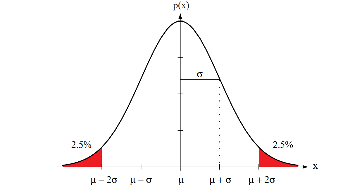
Figure 2.7: a univariate normal has roughly of its area inside ; the peak value is .
The Multivariate Normal Density
where the mean vector and the covariance matrix replace the two scalars of the univariate case.
Formal Definitions
The expected value of a vector or a matrix is taken componentwise: with the -th component of and the -th component of ,
Properties of the Covariance Matrix
is symmetric and positive semidefinite; we assume it is positive definite, so that and the inverse exists.
The diagonal element is the variance of , that is .
The off-diagonal element is the covariance of and ; for the length and weight of a population of fish we would expect it to be positive.
If and are statistically independent then ; if all off-diagonal elements vanish, factorises into the product of univariate normal densities.
Parameters and Geometry
The multivariate normal is completely specified by parameters: the elements of and the independent elements of .
Samples fall in a single cluster whose centre is and whose shape is . The loci of constant density are the hyperellipsoids
whose principal axes are the eigenvectors of and whose axis lengths follow from the eigenvalues. The quadratic form itself is the squared Mahalanobis distance from to : contours of constant density are contours of constant Mahalanobis distance, and the volume they enclose measures the scatter of the samples.
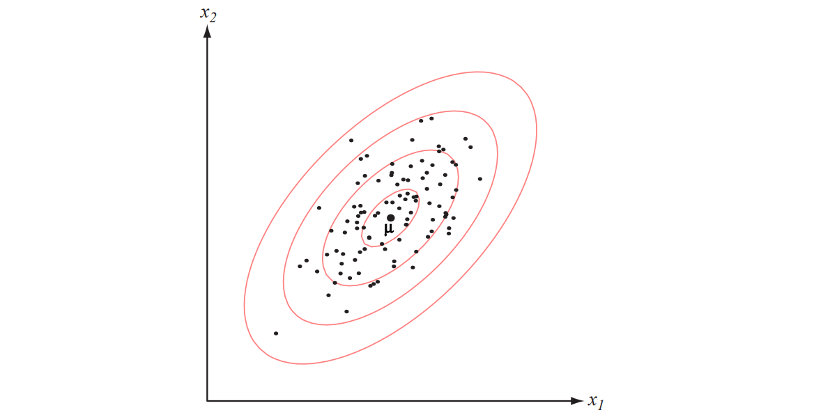
Figure 2.9: samples from a two-dimensional Gaussian lie in a cloud centred on ; the red ellipses are lines of equal probability density.
Discriminant Functions for Normal Densities
Case 1: Isotropic Covariance, 
The simplest case: all classes share the same spherical covariance. Then and , so the density and its logarithm are
Substituting into , and dropping the term because it is the same for every class:
With equal priors the rule is “assign to the nearest mean”, with the Euclidean distance scaled by . With unequal priors, a point that is equally near two means is given to the a priori more likely class, because is the tie-breaker.
The Linear Form and the Boundary
Expanding the quadratic form,
The term does not depend on and can be dropped as an additive constant, which leaves a linear discriminant
where is the threshold (or bias) of class . A classifier built from linear discriminants is a linear machine: its decision surfaces are pieces of hyperplanes, given by for the two classes whose posteriors are largest. For two classes that equation reads
So the boundary is a hyperplane through , orthogonal to — orthogonal, that is, to the line joining the two means. With equal priors is the midpoint and the boundary is the perpendicular bisector of the segment between the means; with unequal priors it slides away from the more likely mean, by an amount that is large when is large compared with and negligible when the means are far apart.
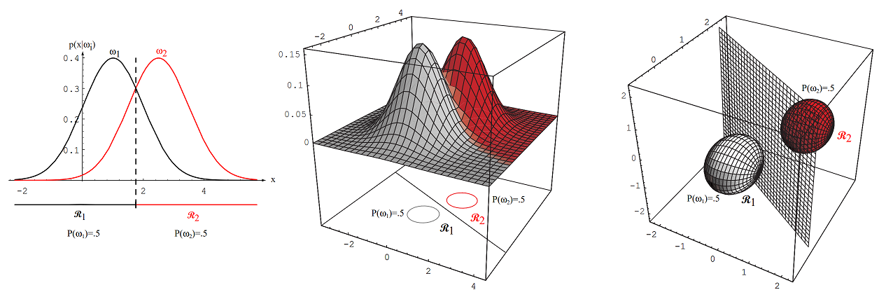
Figure 2.10: with equal isotropic covariances the class regions are separated by a generalised hyperplane of dimensions, perpendicular to the line joining the means.
Minimum Distance Classifier
If all priors are also equal, is an additive constant, and the rule reduces to measuring the Euclidean distance and assigning the nearest mean. This is the minimum distance classifier. Reading each mean as an ideal prototype of its class makes it a template-matching procedure, and it is exactly the nearest-neighbour rule of the previous chapter with one template per class instead of the whole training set.
What a Hyperplane Looks Like in Two Dimensions
The equation says that the vector is orthogonal to for every point of the surface, so:
is a normal to the surface and fixes its orientation;
is one fixed point of the surface;
in the surface is a line, and the equation becomes .
For example, with and the line is . The next cell draws it together with the normal vector.
import matplotlib.pyplot as plt
import numpy as np

# Define the normal vector w and point x0
w = np.array([2, 1])  # Normal vector
x0 = np.array([1, 1])  # Point on the line

# Define the line equation: 2x + y - 3 = 0 => y = -2x + 3
x_values = np.linspace(-5, 5, 100)  # Range of x values
y_values = -2 * x_values + 3  # Corresponding y values

# Plot the line
plt.plot(x_values, y_values, label=r"Line: $2x + y - 3 = 0$")

# Plot the point x0
plt.scatter(x0[0], x0[1], color="red", label=r"Point $\mathbf{x}_0 = (1, 1)$")

# Plot the normal vector w starting from x0
plt.quiver(x0[0], x0[1], w[0], w[1], angles='xy', scale_units='xy', scale=1, color="green", label=r"Normal vector $\mathbf{w} = (2, 1)$")

# Add labels and legend
plt.xlabel("x")
plt.ylabel("y")
plt.axhline(0, color="black", linewidth=0.5)  # x-axis
plt.axvline(0, color="black", linewidth=0.5)  # y-axis
plt.grid(True)
plt.legend()
plt.title("Line and Normal Vector Visualization")
plt.xlim(-5, 5)  # Adjust x-axis limits
plt.ylim(-5, 5)  # Adjust y-axis limits
plt.gca().set_aspect("equal", adjustable="box")  # Equal aspect ratio
plt.show()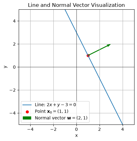
Case 2: Equal but Arbitrary Covariance Matrices, 
When all classes share the same non-spherical covariance, the general discriminant
follows from the Gaussian after dropping and , which are now common to all classes. Expanding the quadratic term (using that is symmetric, so ):
The first term does not depend on and is dropped; what remains is again linear,
so the boundaries are hyperplanes. Setting :
The Geometry of Case 2
Write the boundary as with
The normal points along , which in general is not the direction of : the shared covariance rotates the boundary. Only when is proportional to do we recover Case 1. With equal priors the logarithm vanishes and the boundary passes through , but it is not perpendicular to the line between the means.
The surfaces of constant Mahalanobis distance from the two means are hyperellipsoids of the same shape and orientation, one per class, because is shared. They are linear boundaries only because the quadratic terms cancel in .
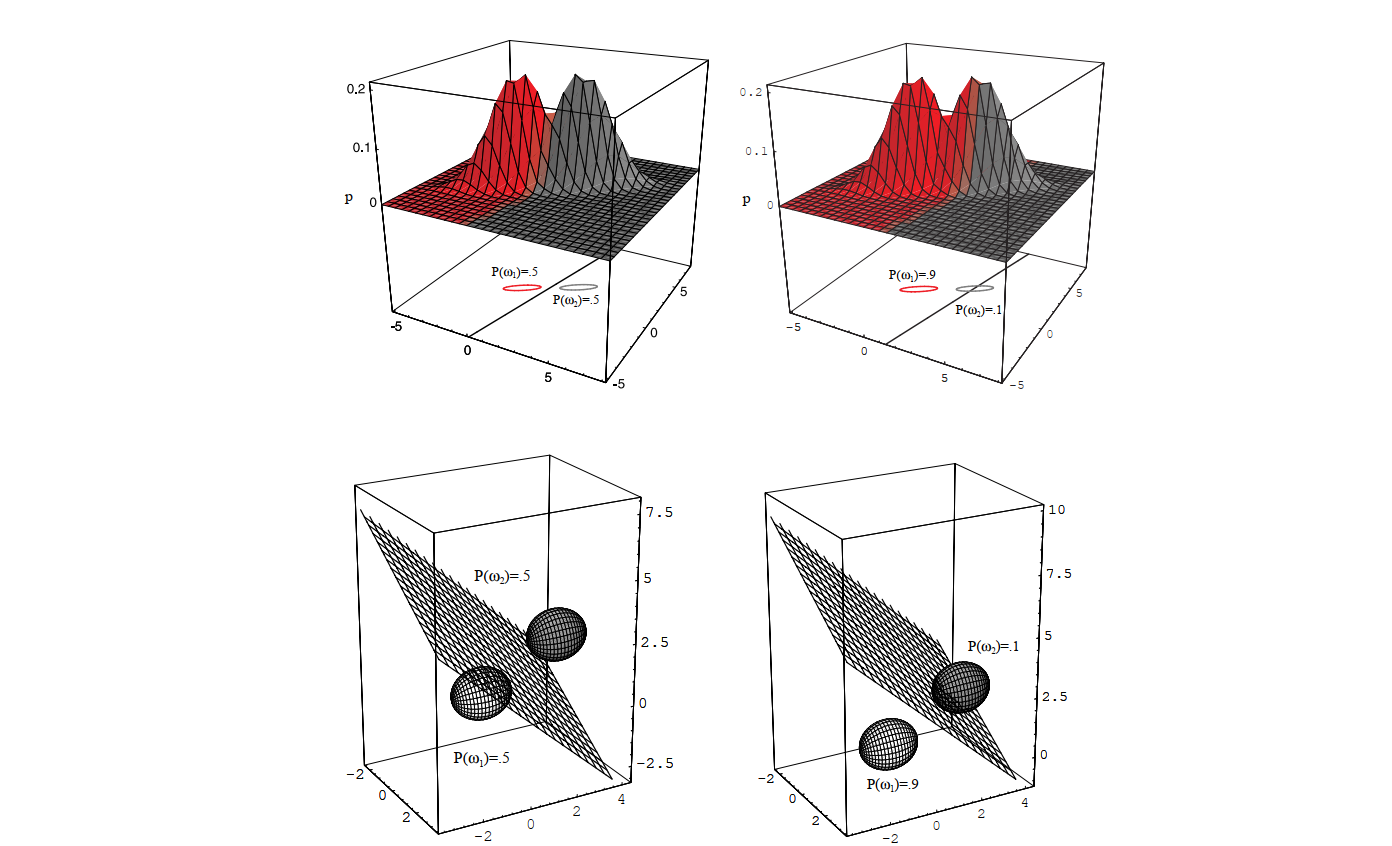
Figure 2.12: equal covariance matrices give linear boundaries that are not necessarily perpendicular to the line joining the means; both classes are shown with the same ellipses of equal density, and the boundary moves with the priors. The next figure shows it sliding as the priors change, for one-, two- and three-dimensional spherical classes.
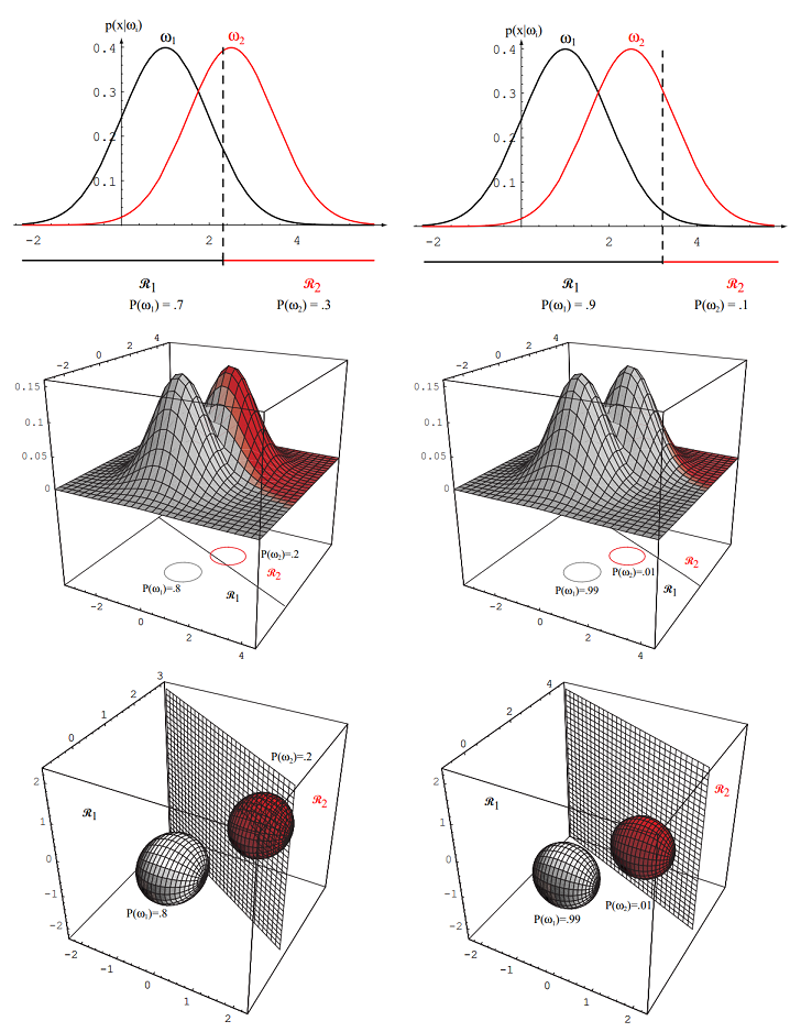
Figure 2.11: as the priors are changed, the decision boundary shifts; for sufficiently disparate priors the boundary will not lie between the means of these 1-, 2- and 3-dimensional spherical Gaussian distributions
Case 3: Arbitrary Covariance Matrices, 
The general case: each class has its own mean and its own covariance . Starting from
and expanding the quadratic form exactly as in Case 2, but now with :
This is a quadratic form in ,
The difference from Case 2 is the term : with unequal covariances the volume of the class matters, and a diffuse class is penalised. The discriminant is now quadratic in and the boundary, given by ,
does not lose its quadratic term, because .
What the Quadratic Boundaries Look Like
A surface of this kind is a hyperquadric — a hyperplane, a pair of hyperplanes, a hypersphere, a hyperellipsoid, a hyperparaboloid or a hyperhyperboloid, depending on the eigenvalues of and on the linear and constant terms. In two dimensions those are a line, a pair of lines, a circle, an ellipse, a parabola and a hyperbola. Every one of these shapes can arise from two Gaussians, and conversely every hyperquadric is the Bayes boundary of some pair of Gaussians.
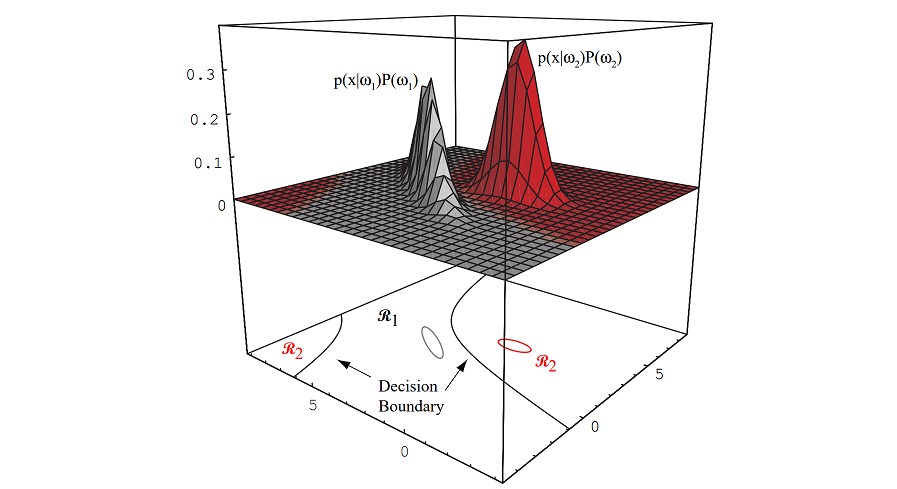
Figure 2.6: a two-dimensional two-category Gaussian classifier with unequal covariances. The two hyperbolas are the boundary, so the decision region is not simply connected — a reminder that “the” boundary may have several branches.
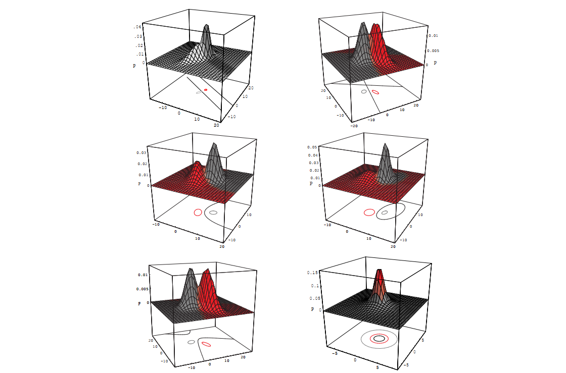
Figure 2.14: arbitrary Gaussians give hyperquadric boundaries; the four panels show an ellipse, a hyperbola, a parabola and a pair of lines.
More Than Two Classes
Extending the result to classes is straightforward, but one has to keep track of which two classes are responsible for each piece of a boundary. Figure 2.16 shows the decision regions of a four-class problem with Gaussian classes: even with four classes the regions are already complicated, and the same theory still governs them.
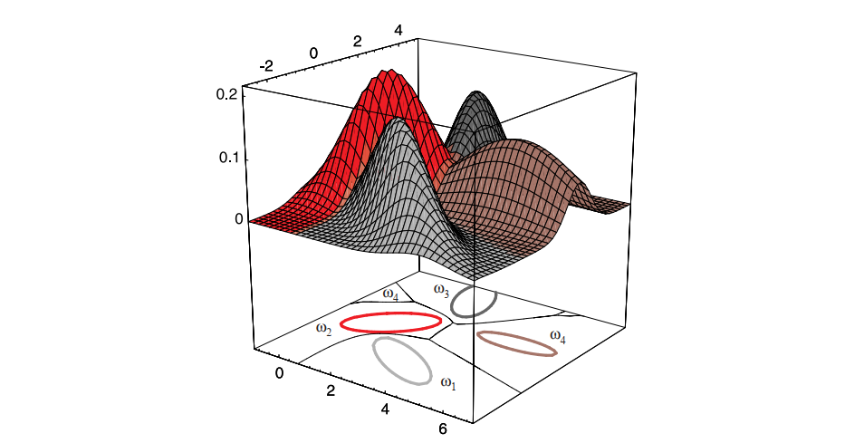
Figure 2.16: the decision regions of four normal distributions.
Exercise: Verifying Case 2 with Scikit-Learn
Objective. Reproduce the Case 2 boundary twice — once from the formula above and once from
GaussianNB — and check that they agree.
Generate data. Two classes, 200 points each, both with covariance and means , .
Theoretical boundary. With , use
and draw the curve on a grid with
plt.contour.Estimated boundary. Fit
GaussianNBon the 200 + 200 points and draw the boundary of its predictions on the same grid.Compare. Plot the two boundaries together, with the points, the line joining the two means, and its perpendicular bisector. The two boundaries should be close but not identical:
GaussianNBestimates and from the sample, while step 2 uses the true parameters. The angle between the boundary normal and the line joining the means is the visible consequence of the shared covariance (Case 2).
Summary
Bayesian decision theory turns probabilities into decisions.
The ingredients are the priors , the class-conditional densities , the posteriors and the evidence , which normalises the posteriors and cancels from every decision.
The general criterion is the conditional risk with a loss matrix ; the zero-one loss reduces it to the minimum error rate rule, “pick the largest posterior”.
Any monotone function of the posterior is a valid discriminant; using the log turns the Gaussian into a quadratic form.
For Gaussian classes there are three regimes. Isotropic and equal covariances give linear discriminants and hyperplane boundaries; arbitrary covariances give quadratic discriminants and hyperquadric boundaries.
The quadratic form inside the Gaussian is the squared Mahalanobis distance, and the three regimes are exactly LDA, LDA with a general , and QDA.
Density parameters are estimated by maximum likelihood; when classes are too small to estimate a full covariance, the naive assumption (independent features) is the usual way out.
References
Duda et al. (2000)
Duda, R. O., Hart, P. E., & Stork, D. G. (2000). Pattern Classification (2nd ed.). Wiley-Interscience, chapter 2.
- Duda, R. O., Hart, P. E., & Stork, D. G. (2000). Pattern Classification (2nd ed.). Wiley-Interscience.