Kernel Regression: From Linear to Nonlinear Modeling

1. Linear Regression Foundation¶

The goal of regression is to predict a continuous output $y$ from input features $\mathbf{x} = (x_1, x_2, ..., x_d)^T$ using a learned function $f$ :

y = f(\mathbf{x}) + \varepsilon

(1)

where $\varepsilon$ represents random noise.

In linear regression, we assume $f$ is linear:

f(\mathbf{x}) = \mathbf{w}^T \mathbf{x}

(2)

(The bias term can be absorbed into $\mathbf{w}$ by adding a constant 1 to $\mathbf{x}$ .)

The parameters $\mathbf{w}$ minimize the sum of squared errors:

\min_{\mathbf{w}} \sum_{i=1}^n (y_i - \mathbf{w}^T \mathbf{x}_i)^2

(3)

2. Kernel Regression: The Core Idea¶

2.1 Why Kernels?¶

Real-world data often has nonlinear patterns that linear models cannot capture. The solution: map each input $\mathbf{x}$ to a higher-dimensional feature space $\phi(\mathbf{x})$ where the relationship becomes linear:

f(\mathbf{x}) = \mathbf{w}^T \phi(\mathbf{x})

(4)

The Challenge: Explicitly computing $\phi(\mathbf{x})$ may be computationally prohibitive or even infinite-dimensional.

The Kernel Trick: Use a kernel function $K$ that computes dot products in the feature space without ever constructing $\phi(\mathbf{x})$ explicitly:

K(\mathbf{x}_i, \mathbf{x}_j) = \langle \phi(\mathbf{x}_i), \phi(\mathbf{x}_j) \rangle

(5)

2.2 The Dual Formulation¶

Using the kernel trick, the regression function becomes a weighted sum of kernel similarities to each training point:

\hat{y}(\mathbf{x}) = \sum_{i=1}^n \alpha_i \, K(\mathbf{x}, \mathbf{x}_i)

(6)

where:

$\alpha_i$ are weights learned from data
$K(\mathbf{x}, \mathbf{x}_i)$ measures similarity between the test point $\mathbf{x}$ and training point $\mathbf{x}_i$

Interpretation: The prediction is a similarity-weighted average of training outputs, where the weights $\alpha_i$ are learned rather than being simple averages.

3. Training: Solving for $\boldsymbol{\alpha}$ ¶

3.1 The Optimization Problem¶

We learn $\alpha_i$ by fitting the training data:

\min_{\boldsymbol{\alpha}} \sum_{j=1}^n \left( y_j - \sum_{i=1}^n \alpha_i K(\mathbf{x}_j, \mathbf{x}_i) \right)^2

(7)

3.2 Matrix Formulation¶

Define:

Kernel matrix $\mathbf{K}$ (size $n \times n$ ): $\mathbf{K}_{ij} = K(\mathbf{x}_i, \mathbf{x}_j)$
Weight vector $\boldsymbol{\alpha} = [\alpha_1, ..., \alpha_n]^T$
Output vector $\mathbf{y} = [y_1, ..., y_n]^T$

For all training points, predictions are:

\hat{\mathbf{y}} = \mathbf{K} \boldsymbol{\alpha}

(8)

The sum of squared errors becomes:

\|\mathbf{y} - \mathbf{K} \boldsymbol{\alpha}\|^2

(9)

3.3 The Solution¶

Taking the derivative and setting to zero:

\frac{\partial}{\partial \boldsymbol{\alpha}} \|\mathbf{y} - \mathbf{K} \boldsymbol{\alpha}\|^2 = -2\mathbf{K}^T(\mathbf{y} - \mathbf{K}\boldsymbol{\alpha}) = 0

(10)

Since $\mathbf{K}$ is symmetric ( $\mathbf{K}^T = \mathbf{K}$ ):

\mathbf{K}(\mathbf{y} - \mathbf{K}\boldsymbol{\alpha}) = 0

(11)

\mathbf{K}\mathbf{y} = \mathbf{K}^2\boldsymbol{\alpha}

(12)

If $\mathbf{K}$ is invertible (positive definite kernel with distinct points), multiply by $\mathbf{K}^{-1}$ :

\mathbf{y} = \mathbf{K}\boldsymbol{\alpha}

(13)

Thus:

\boxed{\boldsymbol{\alpha} = \mathbf{K}^{-1} \mathbf{y}}

(14)

Key Insight: The weights $\boldsymbol{\alpha}$ are chosen so that training predictions perfectly match training outputs ( $\hat{\mathbf{y}}_{\text{train}} = \mathbf{y}$ ). This is exact interpolation.

4. Making Predictions on New Data¶

4.1 Single Test Point¶

For a new test point $\mathbf{x}_{\text{test}}$ (not in training set):

Step 1: Compute kernel similarities between $\mathbf{x}_{\text{test}}$ and all training points:

\mathbf{k}_{\text{test}} = \begin{bmatrix} K(\mathbf{x}_{\text{test}}, \mathbf{x}_1) \\ K(\mathbf{x}_{\text{test}}, \mathbf{x}_2) \\ \vdots \\ K(\mathbf{x}_{\text{test}}, \mathbf{x}_n) \end{bmatrix} \quad \text{(size } n \times 1\text{)}

(15)

Step 2: Make prediction using the same formula:

\hat{y}_{\text{test}} = \sum_{i=1}^n \alpha_i K(\mathbf{x}_{\text{test}}, \mathbf{x}_i) = \mathbf{k}_{\text{test}}^T \boldsymbol{\alpha}

(16)

4.2 Multiple Test Points¶

For $m$ test points $\{\mathbf{x}_{\text{test}}^{(1)}, \dots, \mathbf{x}_{\text{test}}^{(m)}\}$ :

Define $\mathbf{K}_{\text{test}}$ as an $m \times n$ matrix:

[\mathbf{K}_{\text{test}}]_{pj} = K(\mathbf{x}_{\text{test}}^{(p)}, \mathbf{x}_j)

(17)

Then predictions:

\hat{\mathbf{y}}_{\text{test}} = \mathbf{K}_{\text{test}} \, \boldsymbol{\alpha}

(18)

4.3 Training vs. Testing Summary¶

Phase	Input	Prediction	Equals true $y$ ?
Training	$\mathbf{K}$ ( $n \times n$ )	$\hat{\mathbf{y}}_{\text{train}} = \mathbf{K}\boldsymbol{\alpha}$	Yes (exact fit)
Testing	$\mathbf{k}_{\text{test}}$ ( $n \times 1$ )	$\hat{y}_{\text{test}} = \mathbf{k}_{\text{test}}^T \boldsymbol{\alpha}$	No (generalization)

Important: The interpolation property $\hat{\mathbf{y}}_{\text{train}} = \mathbf{y}$ holds only for training data. For test points, predictions are determined by similarity to training points, not by exact matching.

5. The Pseudoinverse Connection¶

5.1 Unified View¶

From the matrix appendix, recall the pseudoinverse $X^+$ solves $X\mathbf{w} = \mathbf{y}$ optimally. For kernel regression, we solve $\mathbf{K}\boldsymbol{\alpha} = \mathbf{y}$ , so:

\boldsymbol{\alpha} = \mathbf{K}^+ \mathbf{y}

(19)

When $\mathbf{K}$ is invertible, $\mathbf{K}^+ = \mathbf{K}^{-1}$ . When $\mathbf{K}$ is singular or ill-conditioned, we use regularization.

5.2 Regularization (Kernel Ridge Regression)¶

In practice, with noisy data, exact interpolation leads to overfitting. Add a ridge penalty $\lambda \|\mathbf{f}\|^2$ :

\min_{\boldsymbol{\alpha}} \|\mathbf{y} - \mathbf{K}\boldsymbol{\alpha}\|^2 + \lambda \boldsymbol{\alpha}^T \mathbf{K} \boldsymbol{\alpha}

(20)

The solution becomes:

\boxed{\boldsymbol{\alpha} = (\mathbf{K} + \lambda \mathbf{I})^{-1} \mathbf{y}}

(21)

This is the kernel ridge regression estimator. The regularization term:

Improves numerical stability (ensures invertibility)
Prevents overfitting by shrinking weights
Controls the smoothness of the prediction function

Practice

import numpy as np
from sklearn.metrics.pairwise import rbf_kernel
import matplotlib.pyplot as plt

# Generate synthetic data
X = np.linspace(-3, 3, 100)[:, None]
y = np.sin(X).ravel() + 0.05*np.random.randn(100)

# Compute RBF kernel (σ=1.0)
K = rbf_kernel(X, X, gamma=0.5)

# Solve for coefficients (with small regularization)
alpha = np.linalg.solve(K + 1e-6*np.eye(len(X)), y)

# Predict new points
X_test = np.linspace(-3.1, 3.1, 200)[:, None]
K_test = rbf_kernel(X_test, X, gamma=0.5)
y_pred = K_test @ alpha

# Plot results
plt.figure(figsize=(8, 4))
plt.scatter(X, y, color='blue', label='Training Data', alpha=0.5)
plt.plot(X_test, y_pred, color='red', label='Kernel Regression')
plt.title('Kernel Regression with RBF Kernel')
plt.legend()
plt.show()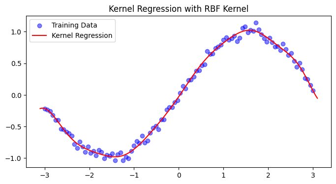

6. The effects of regularization and noise levels on kernel regression¶

import numpy as np
from sklearn.metrics.pairwise import rbf_kernel
import matplotlib.pyplot as plt

# Set random seed for reproducibility
np.random.seed(42)

# --- Generate synthetic data ---
n_train = 50  # Number of training points
X = np.linspace(-3, 3, n_train)[:, None]
true_function = np.sin(X).ravel()  # Underlying smooth function

# --- Create figure with subplots ---
fig, axes = plt.subplots(2, 3, figsize=(15, 10))
fig.suptitle('Kernel Regression: Effects of Regularization and Noise', fontsize=16)

# Parameters to test
noise_levels = [0.0, 0.1]#, 1.0]  # Zero, low, high noise
lambda_regs = [0, 1e-6, 1e-1]    # No regularization, weak, strong

# Store results for comparison
results = {}

for i, noise in enumerate(noise_levels):
    for j, lambda_reg in enumerate(lambda_regs):
        # Generate noisy training data
        y = true_function + noise * np.random.randn(n_train)
        
        # --- Training ---
        # Compute RBF kernel matrix (gamma = 0.5)
        gamma = 0.5
        K = rbf_kernel(X, X, gamma=gamma)
        
        # Solve for alpha with or without regularization
        if lambda_reg == 0:
            # No regularization - direct inversion (may be unstable)
            try:
                alpha = np.linalg.solve(K, y)
                reg_status = "No regularization"
            except np.linalg.LinAlgError:
                alpha = np.linalg.pinv(K) @ y  # Use pseudoinverse if singular
                reg_status = "No regularization (pseudoinverse)"
        else:
            alpha = np.linalg.solve(K + lambda_reg * np.eye(n_train), y)
            reg_status = f"λ = {lambda_reg}"
        
        # --- Testing ---
        X_test = np.linspace(-3.5, 3.5, 300)[:, None]
        K_test = rbf_kernel(X_test, X, gamma=gamma)
        y_pred = K_test @ alpha
        
        # True function on test points
        y_true_test = np.sin(X_test).ravel()
        
        # Calculate test error
        test_mse = np.mean((y_pred - y_true_test)**2)
        
        # --- Plot ---
        ax = axes[i, j]
        ax.scatter(X, y, color='blue', alpha=0.6, s=30, label='Training data')
        ax.plot(X_test, y_true_test, 'k--', linewidth=2, label='True function', alpha=0.7)
        ax.plot(X_test, y_pred, 'r-', linewidth=2, label='Kernel regression')
        ax.set_xlabel('x')
        ax.set_ylabel('y')
        ax.grid(True, alpha=0.3)
        
        # Add title with parameters
        title = f"Noise σ = {noise}\n{reg_status}"
        ax.set_title(title)
        
        # Display MSE in the corner
        ax.text(0.05, 0.95, f'MSE = {test_mse:.4f}', 
                transform=ax.transAxes, verticalalignment='top',
                bbox=dict(boxstyle='round', facecolor='wheat', alpha=0.5))
        
        # Add legend only for first plot
        if i == 0 and j == 0:
            ax.legend(loc='upper right')
        
        # Store results
        results[(noise, lambda_reg)] = {'mse': test_mse, 'alpha': alpha}

plt.tight_layout()
plt.show()


# --- Print summary table ---
print("\n" + "="*70)
print("SUMMARY: Test MSE for different noise levels and regularization")
print("="*70)
print(f"{'Noise σ':<10} {'λ = 0':<20} {'λ = 1e-6':<20} {'λ = 0.1':<20}")
print("-"*70)

for noise in noise_levels:
    row = f"{noise:<10}"
    for lambda_reg in lambda_regs:
        mse = results[(noise, lambda_reg)]['mse']
        row += f"{mse:<20.6f}"
    print(row)
print("="*70)

# --- Interpretation guide ---
print("\n" + "📊 INTERPRETATION GUIDE 📊".center(70))
print("="*70)
print("1. NOISE σ = 0 (No noise):")
print("   - λ = 0: Perfect fit (MSE ≈ 0) - model interpolates exactly")
print("   - λ > 0: Slight bias introduced, but still good fit")
print("\n2. NOISE σ = 0.1 (Low noise):")
print("   - λ = 0: May overfit slightly, capturing noise patterns")
print("   - λ = 1e-6: Balances fit and smoothness")
print("   - λ = 0.1: May underfit (too smooth)")
print("\n💡 KEY INSIGHT:")
print("   - More noise → need stronger regularization (larger λ)")
print("   - No noise → λ = 0 gives perfect interpolation")
print("   - Too much regularization → underfitting (bias)")
print("   - Too little regularization → overfitting (variance)")
print("="*70)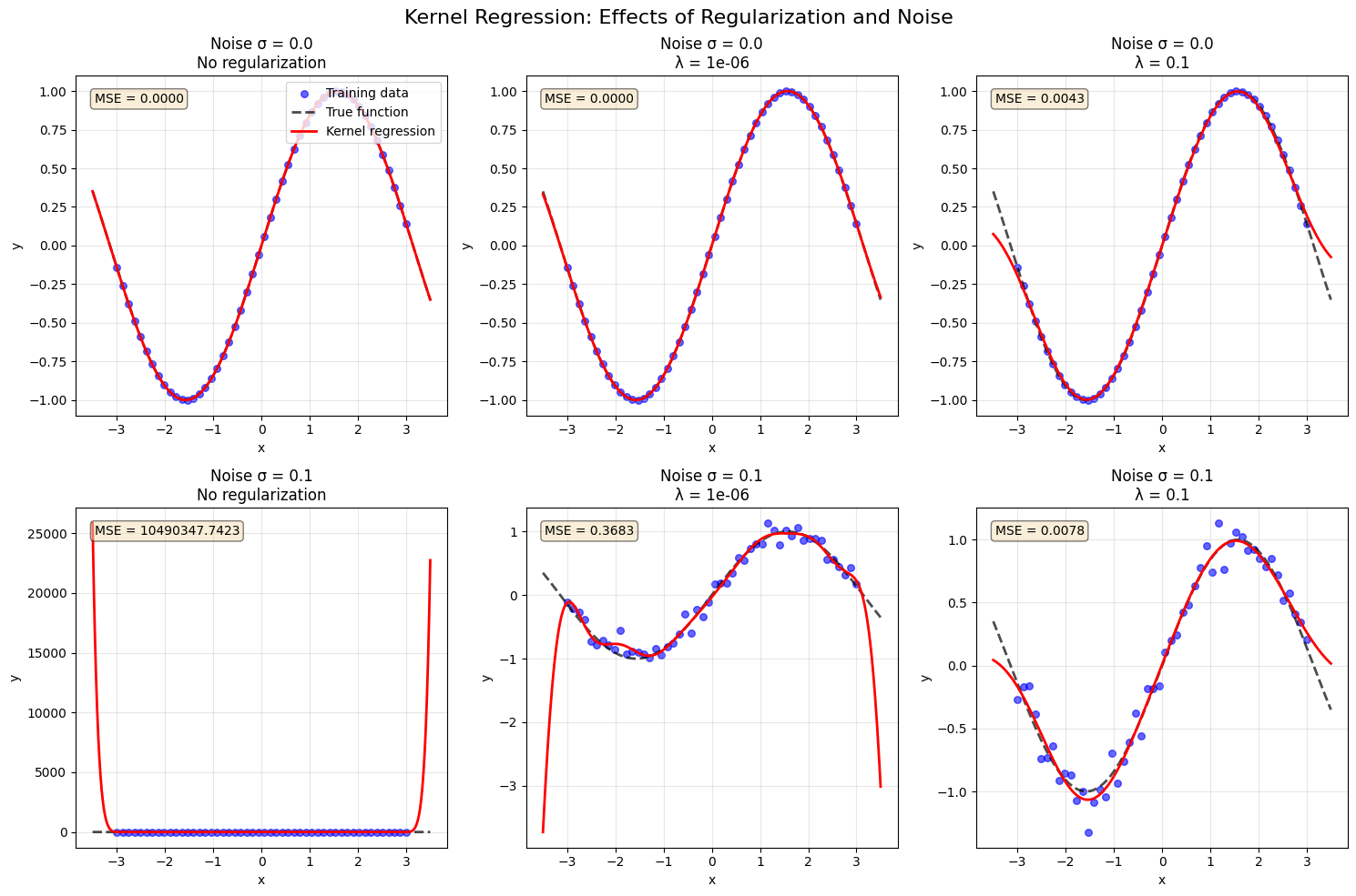


======================================================================
SUMMARY: Test MSE for different noise levels and regularization
======================================================================
Noise σ    λ = 0                λ = 1e-6             λ = 0.1             
----------------------------------------------------------------------
0.0       0.000000            0.000008            0.004277            
0.1       10490347.742265     0.368313            0.007773            
======================================================================

                       📊 INTERPRETATION GUIDE 📊                       
======================================================================
1. NOISE σ = 0 (No noise):
   - λ = 0: Perfect fit (MSE ≈ 0) - model interpolates exactly
   - λ > 0: Slight bias introduced, but still good fit

2. NOISE σ = 0.1 (Low noise):
   - λ = 0: May overfit slightly, capturing noise patterns
   - λ = 1e-6: Balances fit and smoothness
   - λ = 0.1: May underfit (too smooth)

💡 KEY INSIGHT:
   - More noise → need stronger regularization (larger λ)
   - No noise → λ = 0 gives perfect interpolation
   - Too much regularization → underfitting (bias)
   - Too little regularization → overfitting (variance)
======================================================================

8. Primal vs. Dual Perspective¶

8.1 Two Forms of the Solution¶

In standard linear regression with features $\mathbf{X}$ , the weight vector can be expressed in two equivalent ways:

Primal Form (feature space):

\mathbf{w} = (\mathbf{X}^T \mathbf{X})^{-1} \mathbf{X}^T \mathbf{y}

(22)

Dual Form (sample space):

\mathbf{w} = \mathbf{X}^T (\mathbf{X} \mathbf{X}^T)^{-1} \mathbf{y}

(23)

Both yield the same predictions when $\mathbf{X}$ has full column rank.

8.2 Why the Dual Form Matters for Kernels¶

The dual form reveals that $\mathbf{w}$ is a linear combination of training samples:

\mathbf{w} = \sum_{i=1}^n \alpha_i \mathbf{x}_i, \quad \text{where} \quad \boldsymbol{\alpha} = (\mathbf{X} \mathbf{X}^T)^{-1} \mathbf{y}

(24)

When we map to feature space $\phi(\mathbf{x})$ , this becomes:

\mathbf{w} = \sum_{i=1}^n \alpha_i \phi(\mathbf{x}_i), \quad \text{with} \quad \boldsymbol{\alpha} = (\mathbf{K})^{-1} \mathbf{y}

(25)

where $\mathbf{K}_{ij} = \phi(\mathbf{x}_i)^T \phi(\mathbf{x}_j) = K(\mathbf{x}_i, \mathbf{x}_j)$ .

Key insight: The prediction for a new point becomes:

\hat{y}(\mathbf{x}) = \mathbf{w}^T \phi(\mathbf{x}) = \sum_{i=1}^n \alpha_i \phi(\mathbf{x}_i)^T \phi(\mathbf{x}) = \sum_{i=1}^n \alpha_i K(\mathbf{x}_i, \mathbf{x})

(26)

We never need $\phi(\mathbf{x})$ explicitly — only kernel evaluations $K(\mathbf{x}_i, \mathbf{x})$ !

8.3 Computational Trade-offs¶

Scenario	Primal Form	Dual Form
$n \ll d$ (few samples, many features)	Slow (invert $d \times d$ )	Fast (invert $n \times n$ )
$n \gg d$ (many samples, few features)	Fast (invert $d \times d$ )	Slow (invert $n \times n$ )
Nonlinear kernels (RBF, polynomial)	Not applicable	Required (kernel trick)

Example: RBF kernel with $n=1000$ samples effectively uses infinite-dimensional features ( $d = \infty$ ):

Primal form impossible (cannot compute $\phi(\mathbf{x})$ explicitly)
Dual form works with $1000 \times 1000$ kernel matrix

9. Key Takeaways¶

Kernel regression enables nonlinear fitting by implicitly mapping data to high-dimensional spaces
The dual formulation expresses predictions as weighted sums of kernel similarities:
$\hat{y}(\mathbf{x}) = \sum_{i=1}^n \alpha_i K(\mathbf{x}, \mathbf{x}_i)$
(27)
Training solves $\boldsymbol{\alpha} = \mathbf{K}^{-1}\mathbf{y}$ (unregularized) or $\boldsymbol{\alpha} = (\mathbf{K} + \lambda\mathbf{I})^{-1}\mathbf{y}$ (regularized)
Testing uses $\hat{y}_{\text{test}} = \mathbf{k}_{\text{test}}^T \boldsymbol{\alpha}$ , where $\mathbf{k}_{\text{test}}$ contains similarities between test and training points
Regularization ( $\lambda > 0$ ) is essential for:
- Numerical stability (ensuring $\mathbf{K} + \lambda\mathbf{I}$ is invertible)
- Preventing overfitting to noise
Kernel choice controls model flexibility:
- Linear kernel $\rightarrow$ standard linear regression
- RBF kernel $\rightarrow$ smooth, local approximation
- Polynomial kernel $\rightarrow$ interaction terms up to degree $d$