Feature Maps: Bridging to Kernel Methods

Feature Maps: Bridging to Kernel Methods
1. Introduction to Feature Maps
A feature map transforms input data into a higher-dimensional space:
Key Motivation: Enable linear models to solve non-linear problems by:
Explicit mapping for classification/clustering
Basis expansion for regression
For advanced feature creation techniques, see Feature-Engine’s MathFeatures.
Source
import numpy as np
import matplotlib.pyplot as plt
from sklearn.datasets import make_circles
from sklearn.linear_model import Perceptron
from sklearn.cluster import KMeans
from mpl_toolkits.mplot3d import Axes3D

# 1. Generate Two-Ring Dataset
X, y = make_circles(n_samples=800, noise=0.07, factor=0.4, random_state=42)

# Create a figure with two subplots side-by-side
fig, axes = plt.subplots(1, 2, figsize=(15, 6)) # Adjusted figsize for better side-by-side view
# 2. Visualize Original 2D Data (on the first subplot)
axes[0].scatter(X[y == 0, 0], X[y == 0, 1], color='red', alpha=0.6, label='Class 0')
axes[0].scatter(X[y == 1, 0], X[y == 1, 1], color='blue', alpha=0.6, label='Class 1')
axes[0].set_title("Two-Ring Dataset in 2D Space")
axes[0].set_xlabel("Feature 1")
axes[0].set_ylabel("Feature 2")
axes[0].legend()
axes[0].grid(True)
# 3. Apply Perceptron (Linear Classifier)
perceptron = Perceptron(max_iter=1000, random_state=42)
perceptron.fit(X, y)

# Create decision boundary grid
xx, yy = np.meshgrid(np.linspace(-1.5, 1.5, 200), np.linspace(-1.5, 1.5, 200))
Z = perceptron.decision_function(np.c_[xx.ravel(), yy.ravel()])
Z = Z.reshape(xx.shape)

# Plot Perceptron Classification (on the second subplot)
axes[1].contourf(xx, yy, Z, levels=[-1, 0, 1], alpha=0.4, cmap='RdBu')
axes[1].scatter(X[y == 0, 0], X[y == 0, 1], color='red', alpha=0.6, label='Class 0')
axes[1].scatter(X[y == 1, 0], X[y == 1, 1], color='blue', alpha=0.6, label='Class 1')
axes[1].set_title("Perceptron Classification in 2D (Fails to Separate)")
axes[1].set_xlabel("Feature 1")
axes[1].set_ylabel("Feature 2")
axes[1].legend()

# Adjust layout and display the combined plot
plt.tight_layout()
plt.show()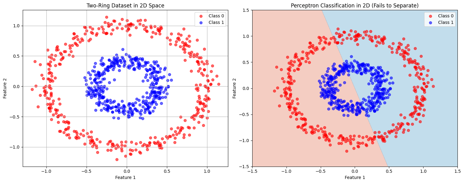
The map makes classes linearly separable by converting radial distance to a linear feature.
# Transform to 3D (z = x² + y²)
X_3d = np.column_stack((X[:, 0], X[:, 1], X[:, 0]**2 + X[:, 1]**2))

# Perceptron in 3D
perceptron.fit(X_3d, y)
Output
Source
import matplotlib.pyplot as plt
# %matplotlib notebook
# Plot in 3D
fig = plt.figure(figsize=(10, 7))
ax = fig.add_subplot(111, projection='3d')
ax.scatter(X_3d[y==0, 0], X_3d[y==0, 1], X_3d[y==0, 2],
           color='red', label='Class 0', alpha=0.6, s=20)
ax.scatter(X_3d[y==1, 0], X_3d[y==1, 1], X_3d[y==1, 2],
           color='blue', label='Class 1', alpha=0.6, s=20)

# Add optimal separating plane
xx, yy = np.meshgrid(np.linspace(-1.5, 1.5, 20), np.linspace(-1.5, 1.5, 20))
zz = np.full(xx.shape, 0.5)  # Plane at z=0.5 (optimal boundary)
ax.plot_surface(xx, yy, zz, alpha=0.3, color='green')

ax.set_title("Linearly Separable in 3D Space")
ax.set_xlabel("Feature 1 (x)")
ax.set_ylabel("Feature 2 (y)")
ax.set_zlabel("Feature 3 (x² + y²)")
ax.legend()
plt.show()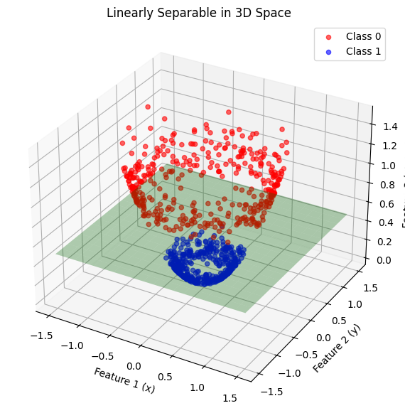
Source
import plotly.graph_objects as go

fig = go.Figure(data=[
    go.Scatter3d(
        x=X_3d[y==0, 0], y=X_3d[y==0, 1], z=X_3d[y==0, 2],
        mode='markers', marker=dict(size=3, color='red'), name='Class 0'
    ),
    go.Scatter3d(
        x=X_3d[y==1, 0], y=X_3d[y==1, 1], z=X_3d[y==1, 2],
        mode='markers', marker=dict(size=3, color='blue'), name='Class 1'
    ),
    go.Surface(
        x=xx, y=yy, z=zz, opacity=0.3, colorscale='Greens', showscale=False
    )
])

fig.update_layout(
    title="Linearly Separable in 3D Space (Interactive)",
    scene=dict(
        xaxis_title='Feature 1 (x)',
        yaxis_title='Feature 2 (y)',
        zaxis_title='Feature 3 (x² + y²)'
    )
)
fig.show()3. Clustering: Two-Ring Problem
Source
# Apply K-Means Clustering in 2D
kmeans = KMeans(n_clusters=2, random_state=42)
kmeans.fit(X)
cluster_labels = kmeans.labels_

fig = plt.figure(figsize=(12, 6))
ax1 = fig.add_subplot(121)
# plt.figure(figsize=(10, 5))
ax1.scatter(X[cluster_labels == 0, 0], X[cluster_labels == 0, 1], color='red', alpha=0.6, label='Cluster 0')
ax1.scatter(X[cluster_labels == 1, 0], X[cluster_labels == 1, 1], color='blue', alpha=0.6, label='Cluster 1')
ax1.legend()

# Transform to 3D (z = x² + y²)
X_3d = np.column_stack((X[:, 0], X[:, 1], X[:, 0]**2 + X[:, 1]**2))
# 7. K-Means in 3D
# kmeans_3d = KMeans(n_clusters=2, random_state=42)
kmeans.fit(X_3d)
cluster_labels_3d = kmeans.labels_

# K-Means results in 3D
ax2 = fig.add_subplot(122, projection='3d')
ax2.scatter(X_3d[cluster_labels_3d == 0, 0],
            X_3d[cluster_labels_3d == 0, 1],
            X_3d[cluster_labels_3d == 0, 2], color='red', alpha=0.6, label='Cluster 0')
ax2.scatter(X_3d[cluster_labels_3d == 1, 0],
            X_3d[cluster_labels_3d == 1, 1],
            X_3d[cluster_labels_3d == 1, 2], color='blue', alpha=0.6, label='Cluster 1')
ax2.set_title("K-Means Clustering in 3D (Correct Separation)")
ax2.set_xlabel("Feature 1")
ax2.set_ylabel("Feature 2")
ax2.set_zlabel("x² + y²")
ax2.legend()

plt.tight_layout()
plt.show()
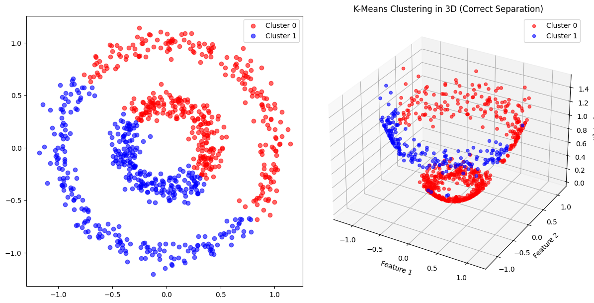
Regression Example: Using Feature Maps for Non-Linear Data
Goal: To demonstrate how mapping features to a higher-dimensional space can allow a linear model to fit non-linear data.
Motivation: Standard linear regression models assume a linear relationship between the features (independent variables) and the target (dependent variable). What happens when the underlying relationship is non-linear? A simple linear model will perform poorly.
Consider a scenario where the data follows a curve, for example, a quadratic relationship. A straight line (from linear regression) won’t capture this curve effectively.
Solution Idea: We can transform the original features into a higher-dimensional space where the relationship becomes linear. This transformation is called a feature map, denoted by Φ.
Let’s illustrate this with an example.
1. Generating Non-Linear Data
We’ll create synthetic data where y depends quadratically on x, plus some random noise to make it more realistic.
Source
import numpy as np
import matplotlib.pyplot as plt
from sklearn.linear_model import LinearRegression
from sklearn.preprocessing import PolynomialFeatures

np.random.seed(42)

# Generate data points
m = 100 # number of samples
X = 6 * np.random.rand(m, 1) - 3 # Feature values between -3 and 3
y = 0.5 * X**2 + X + 2 + np.random.randn(m, 1) # Quadratic relationship + noise

# Visualize the generated data
plt.figure(figsize=(8, 6))
plt.scatter(X, y, alpha=0.7)
plt.title("Generated Non-Linear Data (Quadratic Relationship)")
plt.xlabel("Feature (x)")
plt.ylabel("Target (y)")
plt.grid(True)
plt.show()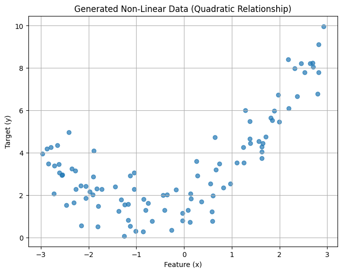
As you can see, the data clearly follows a curve, not a straight line.
2. Attempting Simple Linear Regression (Original Space)
Let’s see how a standard linear regression model performs on this data without any feature transformation.
Source
# Train a simple linear regression model
lin_reg = LinearRegression()
lin_reg.fit(X, y)

# Make predictions
X_new = np.linspace(-3, 3, 100).reshape(100, 1) # Points for plotting the line
y_pred_linear = lin_reg.predict(X_new)

# Visualize the fit
plt.figure(figsize=(8, 6))
plt.scatter(X, y, alpha=0.7, label="Data Points")
plt.plot(X_new, y_pred_linear, "r-", linewidth=2, label="Linear Regression Fit")
plt.title("Simple Linear Regression on Non-Linear Data")
plt.xlabel("Feature (x)")
plt.ylabel("Target (y)")
plt.legend()
plt.grid(True)
plt.show()

print(f"Linear Regression Score (R^2): {lin_reg.score(X, y):.4f}")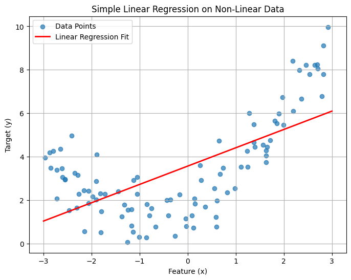
Linear Regression Score (R^2): 0.4260
The linear model tries its best to fit a straight line through the curved data, but it’s clearly a poor fit. The R² score will likely be low, indicating that the model doesn’t explain much of the variance in the data.
3. Applying a Feature Map (Polynomial Features)
Now, let’s apply a feature map. Since we know the underlying relationship is quadratic (y ≈ ax² + bx + c), a suitable feature map Φ would transform our single feature x into two features: x and x².
So, Φ(x) = [x, x²].
We can achieve this using Scikit-Learn’s PolynomialFeatures.
# Create polynomial features (degree=2 includes x and x^2)
# include_bias=False because LinearRegression handles the intercept (bias) term
poly_features = PolynomialFeatures(degree=2, include_bias=False)
X_poly = poly_features.fit_transform(X)

# Display the original feature and the transformed features for the first few samples
print("Original X (first 5 samples):\n", X[:5])
print("\nTransformed X_poly (first 5 samples) [x, x^2]:\n", X_poly[:5])
Original X (first 5 samples):
[[-0.75275929]
[ 2.70428584]
[ 1.39196365]
[ 0.59195091]
[-2.06388816]]
Transformed X_poly (first 5 samples) [x, x^2]:
[[-0.75275929 0.56664654]
[ 2.70428584 7.3131619 ]
[ 1.39196365 1.93756281]
[ 0.59195091 0.35040587]
[-2.06388816 4.25963433]]
Notice that our data is now represented in a 2-dimensional feature space [x, x²].
4. Linear Regression in the Higher-Dimensional Feature Space
Now, we train a linear regression model, but using the transformed features (X_poly). The model will learn weights for both x and x², effectively fitting a model of the form:
y = w₁*x + w₂*x² + b
where w₁, w₂ are the weights (coefficients) and b is the intercept (bias). This is a linear model with respect to the new features x and x².
Original linear model:
A transformation that maps features to higher dimensions:
New model becomes:
For p=1, degree=2:
Source
# Train a linear regression model on the polynomial features
poly_lin_reg = LinearRegression()
poly_lin_reg.fit(X_poly, y)

# Make predictions using the polynomial model
X_new_poly = poly_features.transform(X_new) # Transform the plotting points
y_pred_poly = poly_lin_reg.predict(X_new_poly)

# Visualize the fit
plt.figure(figsize=(8, 6))
plt.scatter(X, y, alpha=0.7, label="Data Points")
plt.plot(X_new, y_pred_poly, "r-", linewidth=2, label="Polynomial Regression Fit (Linear in Feature Space)")
plt.title("Linear Regression on Transformed (Polynomial) Features")
plt.xlabel("Feature (x)")
plt.ylabel("Target (y)")
plt.legend()
plt.grid(True)
plt.show()

print(f"Polynomial Regression Score (R^2): {poly_lin_reg.score(X_poly, y):.4f}")
# Display the learned coefficients (w1 for x, w2 for x^2) and intercept (b)
print(f"Coefficients (w1, w2): {poly_lin_reg.coef_}")
print(f"Intercept (b): {poly_lin_reg.intercept_}")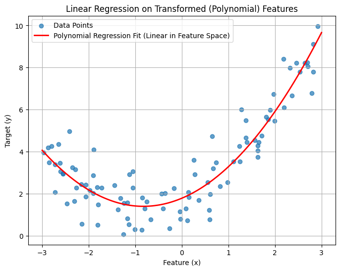
Polynomial Regression Score (R^2): 0.8525
Coefficients (w1, w2): [[0.93366893 0.56456263]]
Intercept (b): [1.78134581]
5. Conclusion
By mapping the original single feature x to a higher-dimensional space [x, x²], we enabled a standard linear regression model to perfectly capture the non-linear (quadratic) relationship present in the data. The resulting fit is much better, as indicated visually and by the significantly higher R² score.
This example illustrates the power of feature maps: transforming data into a space where linear models can become effective, even if the original relationship was non-linear.
Transition to Kernel Trick: While this explicit feature mapping works well for low-dimensional data and simple transformations, calculating and storing these higher-dimensional features can become computationally expensive or even infeasible if the original data or the target feature space is very high-dimensional (e.g., using polynomial features of a very high degree or other complex maps). The Kernel Trick provides a mathematical shortcut to achieve the same result as working in the high-dimensional feature space without explicitly computing the coordinates of the data in that space. It allows algorithms that only depend on dot products between data points (like Support Vector Machines) to operate implicitly in the high-dimensional feature space, making complex mappings computationally tractable. This regression example helps build the intuition for why such implicit mappings are desirable.
Notebook Cell
For modern approaches, see Dynamic and Adaptive Feature Generation with LLM.