import numpy as np
import matplotlib.pyplot as plt
import seaborn as sns

# Plot style
sns.set()
%pylab inline
pylab.rcParams['figure.figsize'] = (4, 4)

Populating the interactive namespace from numpy and matplotlib

The Trace Operator¶

This chapter is very light! I can assure you that you will read it in 1 minute! It is nice after the last two chapters that were quite big! We will see what is the Trace of a matrix. It will be needed for the last chapter on the Principal Component Analysis (PCA).

The Trace Operator¶

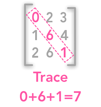The trace of matrix

The trace is the sum of all values in the diagonal of a square matrix.

\boldsymbol{A}= \begin{bmatrix} 2 & 9 & 8 \\\\ 4 & 7 & 1 \\\\ 8 & 2 & 5 \end{bmatrix}

(1)

\mathrm{Tr}(\boldsymbol{A}) = 2 + 7 + 5 = 14

(2)

Numpy provides the function trace() to calculate it:

A = np.array([[2, 9, 8], [4, 7, 1], [8, 2, 5]])
A

array([[2, 9, 8],
       [4, 7, 1],
       [8, 2, 5]])

A_tr = np.trace(A)
A_tr

14

GoodFellow et al. explain that the trace can be used to specify the Frobenius norm of a matrix (see 2.5). The Frobenius norm is the equivalent of the $L^2$ norm for matrices. It is defined by:

\left\lVert \boldsymbol{A} \right\rVert_F=\sqrt{\sum_{i,j}A^2_{i,j}}

(3)

Take the square of all elements and sum them. Take the square root of the result. This norm can also be calculated with:

\left\lVert \boldsymbol{A} \right\rVert_F=\sqrt{\mathrm{Tr}({\boldsymbol{AA}^T})}

(4)

We can check this. The first way to compute the norm can be done with the simple command np.linalg.norm():

np.linalg.norm(A)

17.549928774784245

The Frobenius norm of $\boldsymbol{A}$ is 17.549928774784245.

With the trace the result is identical:

np.sqrt(np.trace(A.dot(A.T)))

17.549928774784245

Since the transposition of a matrix doesn’t change the diagonal, the trace of the matrix is equal to the trace of its transpose:

\mathrm{Tr}(\boldsymbol{A})=\mathrm{Tr}(\boldsymbol{A}^T)

(5)

Trace of a product¶

\mathrm{Tr}(\boldsymbol{ABC}) = \mathrm{Tr}(\boldsymbol{CAB}) = \mathrm{Tr}(\boldsymbol{BCA})

(6)

Example 1.¶

Let’s see an example of this property.

\boldsymbol{A}= \begin{bmatrix} 4 & 12 \\\\ 7 & 6 \end{bmatrix}

(7)

\boldsymbol{B}= \begin{bmatrix} 1 & -3 \\\\ 4 & 3 \end{bmatrix}

(8)

\boldsymbol{C}= \begin{bmatrix} 6 & 6 \\\\ 2 & 5 \end{bmatrix}

(9)

A = np.array([[4, 12], [7, 6]])
B = np.array([[1, -3], [4, 3]])
C = np.array([[6, 6], [2, 5]])

np.trace(A.dot(B).dot(C))

531

np.trace(C.dot(A).dot(B))

531

np.trace(B.dot(C).dot(A))

531

\boldsymbol{ABC}= \begin{bmatrix} 360 & 432 \\\\ 180 & 171 \end{bmatrix}

(10)

\boldsymbol{CAB}= \begin{bmatrix} 498 & 126 \\\\ 259 & 33 \end{bmatrix}

(11)

\boldsymbol{BCA}= \begin{bmatrix} -63 & -54 \\\\ 393 & 594 \end{bmatrix}

(12)

\mathrm{Tr}(\boldsymbol{ABC}) = \mathrm{Tr}(\boldsymbol{CAB}) = \mathrm{Tr}(\boldsymbol{BCA}) = 531

(13)

References¶

Trace (linear algebra) - Wikipedia

Numpy Trace operator