Special Kinds of Matrices and Vectors
import numpy as np
import matplotlib.pyplot as plt
import seaborn as sns
# Plot parameters
sns.set()
%pylab inline
pylab.rcParams['figure.figsize'] = (4, 4)
plt.rcParams['xtick.major.size'] = 0
plt.rcParams['ytick.major.size'] = 0
# Avoid inaccurate floating values (for inverse matrices in dot product for instance)
# See https://stackoverflow.com/questions/24537791/numpy-matrix-inversion-rounding-errors
np.set_printoptions(suppress=True)Populating the interactive namespace from numpy and matplotlib
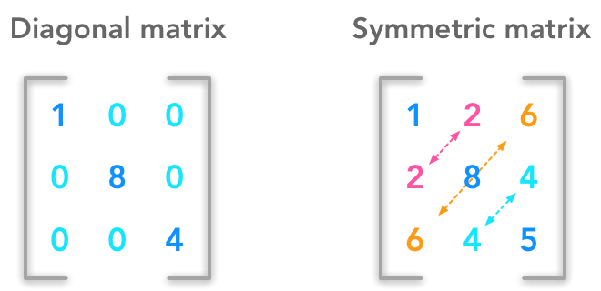
Special Kinds of Matrices and Vectors ¶ We have seen in previous sections some interesting kind of matrices. We will see other type of vectors and matrices in this chapter. It is not a big chapter but it is important to understand the next ones.
Example of diagonal and symmetric matrices
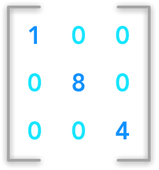
Diagonal matrices ¶ Example of a diagonal matrix
A matrix A i , j \boldsymbol{A}_{i,j} A i , j i = j i=j i = j
Example 1. ¶ D = [ 2 0 0 0 0 4 0 0 0 0 3 0 0 0 0 1 ] \boldsymbol{D}=
\begin{bmatrix}
2 & 0 & 0 & 0\\\\
0 & 4 & 0 & 0\\\\
0 & 0 & 3 & 0\\\\
0 & 0 & 0 & 1
\end{bmatrix} D = ⎣ ⎡ 2 0 0 0 0 4 0 0 0 0 3 0 0 0 0 1 ⎦ ⎤ In this case the matrix is also square but there can be non square diagonal matrices.
Example 2. ¶ D = [ 2 0 0 0 4 0 0 0 3 0 0 0 ] \boldsymbol{D}=
\begin{bmatrix}
2 & 0 & 0\\\\
0 & 4 & 0\\\\
0 & 0 & 3\\\\
0 & 0 & 0
\end{bmatrix} D = ⎣ ⎡ 2 0 0 0 0 4 0 0 0 0 3 0 ⎦ ⎤ Or
D = [ 2 0 0 0 0 4 0 0 0 0 3 0 ] \boldsymbol{D}=
\begin{bmatrix}
2 & 0 & 0 & 0\\\\
0 & 4 & 0 & 0\\\\
0 & 0 & 3 & 0
\end{bmatrix} D = ⎣ ⎡ 2 0 0 0 4 0 0 0 3 0 0 0 ⎦ ⎤ The diagonal matrix can be denoted d i a g ( v ) diag(\boldsymbol{v}) d ia g ( v ) v \boldsymbol{v} v
Example 3. ¶ D = [ 2 0 0 0 0 4 0 0 0 0 3 0 0 0 0 1 ] \boldsymbol{D}=
\begin{bmatrix}
2 & 0 & 0 & 0\\\\
0 & 4 & 0 & 0\\\\
0 & 0 & 3 & 0\\\\
0 & 0 & 0 & 1
\end{bmatrix} D = ⎣ ⎡ 2 0 0 0 0 4 0 0 0 0 3 0 0 0 0 1 ⎦ ⎤ In this matrix, v \boldsymbol{v} v
v = [ 2 4 3 1 ] \boldsymbol{v}=
\begin{bmatrix}
2\\\\
4\\\\
3\\\\
1
\end{bmatrix} v = ⎣ ⎡ 2 4 3 1 ⎦ ⎤ The Numpy function diag() can be used to create square diagonal matrices:
v = np.array([2, 4, 3, 1])
np.diag(v)
array([[2, 0, 0, 0],
[0, 4, 0, 0],
[0, 0, 3, 0],
[0, 0, 0, 1]])
The mutliplication between a diagonal matrix and a vector is thus just a ponderation of each element of the vector by v v v
Example 4. ¶ D = [ 2 0 0 0 0 4 0 0 0 0 3 0 0 0 0 1 ] \boldsymbol{D}=
\begin{bmatrix}
2 & 0 & 0 & 0\\\\
0 & 4 & 0 & 0\\\\
0 & 0 & 3 & 0\\\\
0 & 0 & 0 & 1
\end{bmatrix} D = ⎣ ⎡ 2 0 0 0 0 4 0 0 0 0 3 0 0 0 0 1 ⎦ ⎤ and
x = [ 3 2 2 7 ] \boldsymbol{x}=
\begin{bmatrix}
3\\\\
2\\\\
2\\\\
7
\end{bmatrix} x = ⎣ ⎡ 3 2 2 7 ⎦ ⎤ D x = [ 2 0 0 0 0 4 0 0 0 0 3 0 0 0 0 1 ] × [ 3 2 2 7 ] = [ 2 × 3 + 0 × 2 + 0 × 2 + 0 × 7 0 × 3 + 4 × 2 + 0 × 2 + 0 × 7 0 × 3 + 0 × 2 + 3 × 2 + 0 × 7 0 × 3 + 0 × 2 + 0 × 2 + 1 × 7 ] = [ 2 × 3 4 × 2 3 × 2 1 × 7 ] \begin{align*}
&\boldsymbol{Dx}=
\begin{bmatrix}
2 & 0 & 0 & 0\\\\
0 & 4 & 0 & 0\\\\
0 & 0 & 3 & 0\\\\
0 & 0 & 0 & 1
\end{bmatrix} \times
\begin{bmatrix}
3\\\\
2\\\\
2\\\\
7
\end{bmatrix}\\\\
&=\begin{bmatrix}
2\times3 + 0\times2 + 0\times2 + 0\times7\\\\
0\times3 + 4\times2 + 0\times2 + 0\times7\\\\
0\times3 + 0\times2 + 3\times2 + 0\times7\\\\
0\times3 + 0\times2 + 0\times2 + 1\times7
\end{bmatrix}\\\\
&=
\begin{bmatrix}
2\times3\\\\
4\times2\\\\
3\times2\\\\
1\times7
\end{bmatrix}
\end{align*} Dx = ⎣ ⎡ 2 0 0 0 0 4 0 0 0 0 3 0 0 0 0 1 ⎦ ⎤ × ⎣ ⎡ 3 2 2 7 ⎦ ⎤ = ⎣ ⎡ 2 × 3 + 0 × 2 + 0 × 2 + 0 × 7 0 × 3 + 4 × 2 + 0 × 2 + 0 × 7 0 × 3 + 0 × 2 + 3 × 2 + 0 × 7 0 × 3 + 0 × 2 + 0 × 2 + 1 × 7 ⎦ ⎤ = ⎣ ⎡ 2 × 3 4 × 2 3 × 2 1 × 7 ⎦ ⎤ Non square matrices have the same properties:
Example 5. ¶ D = [ 2 0 0 0 4 0 0 0 3 0 0 0 ] \boldsymbol{D}=
\begin{bmatrix}
2 & 0 & 0\\\\
0 & 4 & 0\\\\
0 & 0 & 3\\\\
0 & 0 & 0
\end{bmatrix} D = ⎣ ⎡ 2 0 0 0 0 4 0 0 0 0 3 0 ⎦ ⎤ and
x = [ 3 2 2 ] \boldsymbol{x}=
\begin{bmatrix}
3\\\\
2\\\\
2
\end{bmatrix} x = ⎣ ⎡ 3 2 2 ⎦ ⎤ D x = [ 2 0 0 0 4 0 0 0 3 0 0 0 ] × [ 3 2 2 ] = [ 2 × 3 4 × 2 3 × 2 0 ] \boldsymbol{Dx}=
\begin{bmatrix}
2 & 0 & 0\\\\
0 & 4 & 0\\\\
0 & 0 & 3\\\\
0 & 0 & 0
\end{bmatrix}
\times
\begin{bmatrix}
3\\\\
2\\\\
2
\end{bmatrix}
=
\begin{bmatrix}
2\times3\\\\
4\times2\\\\
3\times2\\\\
0
\end{bmatrix} Dx = ⎣ ⎡ 2 0 0 0 0 4 0 0 0 0 3 0 ⎦ ⎤ × ⎣ ⎡ 3 2 2 ⎦ ⎤ = ⎣ ⎡ 2 × 3 4 × 2 3 × 2 0 ⎦ ⎤ The invert of a square diagonal matrix exists if all entries of the diagonal are non-zeros. If it is the case, the invert is easy to find. Also, the inverse doen’t exist if the matrix is non-square.
D = [ 2 0 0 0 0 4 0 0 0 0 3 0 0 0 0 1 ] \boldsymbol{D}=
\begin{bmatrix}
2 & 0 & 0 & 0\\\\
0 & 4 & 0 & 0\\\\
0 & 0 & 3 & 0\\\\
0 & 0 & 0 & 1
\end{bmatrix} D = ⎣ ⎡ 2 0 0 0 0 4 0 0 0 0 3 0 0 0 0 1 ⎦ ⎤ D − 1 = [ 1 2 0 0 0 0 1 4 0 0 0 0 1 3 0 0 0 0 1 1 ] \boldsymbol{D}^{-1}=
\begin{bmatrix}
\frac{1}{2} & 0 & 0 & 0\\\\
0 & \frac{1}{4} & 0 & 0\\\\
0 & 0 & \frac{1}{3} & 0\\\\
0 & 0 & 0 & \frac{1}{1}
\end{bmatrix} D − 1 = ⎣ ⎡ 2 1 0 0 0 0 4 1 0 0 0 0 3 1 0 0 0 0 1 1 ⎦ ⎤ D = [ 2 0 0 0 0 4 0 0 0 0 3 0 0 0 0 1 ] [ 1 2 0 0 0 0 1 4 0 0 0 0 1 3 0 0 0 0 1 1 ] = [ 1 0 0 0 0 1 0 0 0 0 1 0 0 0 0 1 ] \boldsymbol{D}=
\begin{bmatrix}
2 & 0 & 0 & 0\\\\
0 & 4 & 0 & 0\\\\
0 & 0 & 3 & 0\\\\
0 & 0 & 0 & 1
\end{bmatrix}
\begin{bmatrix}
\frac{1}{2} & 0 & 0 & 0\\\\
0 & \frac{1}{4} & 0 & 0\\\\
0 & 0 & \frac{1}{3} & 0\\\\
0 & 0 & 0 & \frac{1}{1}
\end{bmatrix}=
\begin{bmatrix}
1 & 0 & 0 & 0\\\\
0 & 1 & 0 & 0\\\\
0 & 0 & 1 & 0\\\\
0 & 0 & 0 & 1
\end{bmatrix} D = ⎣ ⎡ 2 0 0 0 0 4 0 0 0 0 3 0 0 0 0 1 ⎦ ⎤ ⎣ ⎡ 2 1 0 0 0 0 4 1 0 0 0 0 3 1 0 0 0 0 1 1 ⎦ ⎤ = ⎣ ⎡ 1 0 0 0 0 1 0 0 0 0 1 0 0 0 0 1 ⎦ ⎤ Let’s check with Numpy that the multiplication of the matrix with its invert gives us the identity matrix:
A = np.array([[2, 0, 0, 0], [0, 4, 0, 0], [0, 0, 3, 0], [0, 0, 0, 1]])
A
array([[2, 0, 0, 0],
[0, 4, 0, 0],
[0, 0, 3, 0],
[0, 0, 0, 1]])
A_inv = np.array([[1/2., 0, 0, 0], [0, 1/4., 0, 0], [0, 0, 1/3., 0], [0, 0, 0, 1/1.]])
A_inv
array([[0.5 , 0. , 0. , 0. ],
[0. , 0.25 , 0. , 0. ],
[0. , 0. , 0.33333333, 0. ],
[0. , 0. , 0. , 1. ]])
array([[1., 0., 0., 0.],
       [0., 1., 0., 0.],
       [0., 0., 1., 0.],
       [0., 0., 0., 1.]])
Great! This gives the identity matrix
Illustration of a symmetric matrix
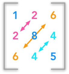
The matrix A A A
A = A T \boldsymbol{A} = \boldsymbol{A}^\text{T} A = A T This concerns only square matrices.
Example 6. ¶ A = [ 2 4 − 1 4 − 8 0 − 1 0 3 ] \boldsymbol{A}=
\begin{bmatrix}
2 & 4 & -1\\\\
4 & -8 & 0\\\\
-1 & 0 & 3
\end{bmatrix} A = ⎣ ⎡ 2 4 − 1 4 − 8 0 − 1 0 3 ⎦ ⎤ A = np.array([[2, 4, -1], [4, -8, 0], [-1, 0, 3]])
Aarray([[ 2, 4, -1],
[ 4, -8, 0],
[-1, 0, 3]])
array([[ 2,  4, -1],
       [ 4, -8,  0],
       [-1,  0,  3]])
Unit vectors ¶ A unit vector is a vector of length equal to 1. It can be denoted by a letter with a hat: u ^ \hat{u} u ^
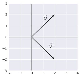
Orthogonal vectors ¶ Two orthogonal vectors are separated by a 90° angle. The dot product of two orthogonal vectors gives 0.
Example 7. ¶ x = [0,0,2,2]
y = [0,0,2,-2]
plt.quiver([x[0], y[0]],
[x[1], y[1]],
[x[2], y[2]],
[x[3], y[3]],
angles='xy', scale_units='xy', scale=1)
plt.xlim(-2, 4)
plt.ylim(-3, 3)
plt.axvline(x=0, color='grey')
plt.axhline(y=0, color='grey')
plt.text(1, 1.5, r'$\vec{u}$', size=18)
plt.text(1.5, -1, r'$\vec{v}$', size=18)
plt.show()
plt.close()x = [ 2 2 ] \boldsymbol{x}=
\begin{bmatrix}
2\\\\
2
\end{bmatrix} x = ⎣ ⎡ 2 2 ⎦ ⎤ and
y = [ 2 − 2 ] \boldsymbol{y}=
\begin{bmatrix}
2\\\\
-2
\end{bmatrix} y = ⎣ ⎡ 2 − 2 ⎦ ⎤ x T y = [ 2 2 ] [ 2 − 2 ] = [ 2 × 2 + 2 × − 2 ] = 0 \boldsymbol{x^\text{T}y}=
\begin{bmatrix}
2 & 2
\end{bmatrix}
\begin{bmatrix}
2\\\\
-2
\end{bmatrix}=
\begin{bmatrix}
2\times2 + 2\times-2
\end{bmatrix}=0 x T y = [ 2 2 ] ⎣ ⎡ 2 − 2 ⎦ ⎤ = [ 2 × 2 + 2 × − 2 ] = 0 In addition, when the norm of orthogonal vectors is the unit norm they are called orthonormal .
It is impossible to have more than n n n R n \mathbb{R}^n R n R 2 \mathbb{R}^2 R 2
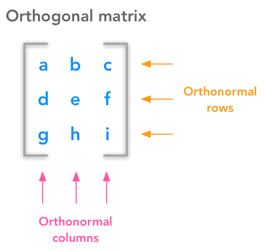
Orthogonal matrices ¶ Orthogonal matrices are important because they have interesting properties. A matrix is orthogonal if columns are mutually orthogonal and have a unit norm (orthonormal) and rows are mutually orthonormal and have unit norm.
Under the hood of an orthogonal matrix
A = [ A 1 , 1 A 1 , 2 A 2 , 1 A 2 , 2 ] \boldsymbol{A}=
\begin{bmatrix}
A_{1,1} & A_{1,2}\\\\
A_{2,1} & A_{2,2}
\end{bmatrix} A = ⎣ ⎡ A 1 , 1 A 2 , 1 A 1 , 2 A 2 , 2 ⎦ ⎤ This means that
[ A 1 , 1 A 2 , 1 ] \begin{bmatrix}
A_{1,1}\\\\
A_{2,1}
\end{bmatrix} ⎣ ⎡ A 1 , 1 A 2 , 1 ⎦ ⎤ and
[ A 1 , 2 A 2 , 2 ] \begin{bmatrix}
A_{1,2}\\\\
A_{2,2}
\end{bmatrix} ⎣ ⎡ A 1 , 2 A 2 , 2 ⎦ ⎤ are orthogonal vectors and also that the rows
[ A 1 , 1 A 1 , 2 ] \begin{bmatrix}
A_{1,1} & A_{1,2}
\end{bmatrix} [ A 1 , 1 A 1 , 2 ] and
[ A 2 , 1 A 2 , 2 ] \begin{bmatrix}
A_{2,1} & A_{2,2}
\end{bmatrix} [ A 2 , 1 A 2 , 2 ] are orthogonal vectors (cf. above for definition of orthogonal vectors).
Property 1: A T A = I \boldsymbol{A^\text{T}A}=\boldsymbol{I} A T A = I ¶ A orthogonal matrix has this property:
A T A = A A T = I \boldsymbol{A^\text{T}A}=\boldsymbol{AA^\text{T}}=\boldsymbol{I} A T A = A A T = I We can see that this statement is true with the following reasoning:
Let’s have the following matrix:
A = [ a b c d ] \boldsymbol{A}=\begin{bmatrix}
a & b\\\\
c & d
\end{bmatrix} A = ⎣ ⎡ a c b d ⎦ ⎤ and thus
A T = [ a c b d ] \boldsymbol{A}^\text{T}=\begin{bmatrix}
a & c\\\\
b & d
\end{bmatrix} A T = ⎣ ⎡ a b c d ⎦ ⎤ Let’s do the product:
A T A = [ a c b d ] [ a b c d ] = [ a a + c c a b + c d a b + c d b b + d d ] = [ a 2 + c 2 a b + c d a b + c d b 2 + d 2 ] \begin{align*}
&\boldsymbol{A^\text{T}A}=\begin{bmatrix}
a & c\\\\
b & d
\end{bmatrix}
\begin{bmatrix}
a & b\\\\
c & d
\end{bmatrix}
=
\begin{bmatrix}
aa + cc & ab + cd\\\\
ab + cd & bb + dd
\end{bmatrix}\\\\
&=
\begin{bmatrix}
a^2 + c^2 & ab + cd\\\\
ab + cd & b^2 + d^2
\end{bmatrix}
\end{align*} A T A = ⎣ ⎡ a b c d ⎦ ⎤ ⎣ ⎡ a c b d ⎦ ⎤ = ⎣ ⎡ aa + cc ab + c d ab + c d bb + dd ⎦ ⎤ = ⎣ ⎡ a 2 + c 2 ab + c d ab + c d b 2 + d 2 ⎦ ⎤ We saw that the norm of the vector [ a c ] \begin{bmatrix}
a & c
\end{bmatrix} [ a c ] a 2 + c 2 a^2+c^2 a 2 + c 2 L 2 L^2 L 2 L 2 L^2 L 2 A \boldsymbol{A} A A \boldsymbol{A} A a 2 + c 2 = 1 a^2+c^2=1 a 2 + c 2 = 1 b 2 + d 2 = 1 b^2+d^2=1 b 2 + d 2 = 1
A T A = [ 1 a b + c d a b + c d 1 ] \boldsymbol{A^\text{T}A}=
\begin{bmatrix}
1 & ab + cd\\\\
ab + cd & 1
\end{bmatrix} A T A = ⎣ ⎡ 1 ab + c d ab + c d 1 ⎦ ⎤ Also, a b + c d ab+cd ab + c d [ a c ] a n d [ b d ] \begin{bmatrix}
a & c
\end{bmatrix} and \begin{bmatrix}
b & d
\end{bmatrix} [ a c ] an d [ b d ]
[ a c ] [ b d ] = a b + c d \begin{bmatrix}
a & c
\end{bmatrix}
\begin{bmatrix}
b\\\\
d
\end{bmatrix}
=
ab+cd [ a c ] ⎣ ⎡ b d ⎦ ⎤ = ab + c d And we know that the columns are orthogonal which means that:
[ a c ] [ b d ] = 0 \begin{bmatrix}
a & c
\end{bmatrix}
\begin{bmatrix}
b\\\\
d
\end{bmatrix}=0 [ a c ] ⎣ ⎡ b d ⎦ ⎤ = 0 We thus have the identity matrix:
A T A = [ 1 0 0 1 ] \boldsymbol{A^\text{T}A}=\begin{bmatrix}
1 & 0\\\\
0 & 1
\end{bmatrix} A T A = ⎣ ⎡ 1 0 0 1 ⎦ ⎤ Property 2: A T = A − 1 \boldsymbol{A}^\text{T}=\boldsymbol{A}^{-1} A T = A − 1 ¶ We can show that if A T A = I \boldsymbol{A^\text{T}A}=\boldsymbol{I} A T A = I A T = A − 1
\boldsymbol{A}^\text{T}=\boldsymbol{A}^{-1} A T = A − 1
If we multiply each side of the equation A T A = I \boldsymbol{A^\text{T}A}=\boldsymbol{I} A T A = I A − 1 \boldsymbol{A}^{-1} A − 1
( A T A ) A − 1 = I A − 1 (\boldsymbol{A^\text{T}A})\boldsymbol{A}^{-1}=\boldsymbol{I}\boldsymbol{A}^{-1} ( A T A ) A − 1 = I A − 1 Recall that a matrix or vector doesn’t change when it is multiplied by the identity matrix. So we have:
( A T A ) A − 1 = A − 1 (\boldsymbol{A^\text{T}A})\boldsymbol{A}^{-1}=\boldsymbol{A}^{-1} ( A T A ) A − 1 = A − 1 We also saw that matrix multiplication is associative so we can remove the parenthesis:
A T A A − 1 = A − 1 \boldsymbol{A^\text{T}A}\boldsymbol{A}^{-1}=\boldsymbol{A}^{-1} A T A A − 1 = A − 1 We also know that A A − 1 = I \boldsymbol{A}\boldsymbol{A}^{-1}=\boldsymbol{I} A A − 1 = I
A T I = A − 1 \boldsymbol{A^\text{T}}\boldsymbol{I}=\boldsymbol{A}^{-1} A T I = A − 1 This shows that
A T = A − 1 \boldsymbol{A}^\text{T}=\boldsymbol{A}^{-1} A T = A − 1 You can refer to this question
Example 8. ¶ Sine and cosine are convenient to create orthogonal matrices. Let’s take the following matrix:
A = [ c o s ( 50 ) − s i n ( 50 ) s i n ( 50 ) c o s ( 50 ) ] \boldsymbol{A}=
\begin{bmatrix}
cos(50) & -sin(50)\\\\
sin(50) & cos(50)
\end{bmatrix} A = ⎣ ⎡ cos ( 50 ) s in ( 50 ) − s in ( 50 ) cos ( 50 ) ⎦ ⎤ A = np.array([[np.cos(50), -np.sin(50)], [np.sin(50), np.cos(50)]])
Aarray([[ 0.96496603, 0.26237485],
[-0.26237485, 0.96496603]])
col0 = A[:, [0]]
col1 = A[:, [1]]
row0 = A[0].reshape(A.shape[1], 1)
row1 = A[1].reshape(A.shape[1], 1)
Let’s check that rows and columns are orthogonal:
Let’s check that
A T A = A A T = I \boldsymbol{A^\text{T}A}=\boldsymbol{AA^\text{T}}=\boldsymbol{I} A T A = A A T = I and thus
A T = A − 1 \boldsymbol{A}^\text{T}=\boldsymbol{A}^{-1} A T = A − 1 array([[1., 0.],
[0., 1.]])
array([[ 0.96496603, -0.26237485],
       [ 0.26237485,  0.96496603]])
array([[ 0.96496603, -0.26237485],
       [ 0.26237485,  0.96496603]])
Everything is correct!
Conclusion ¶ In this chapter we saw different interesting type of matrices with specific properties. It is generally useful to recall them while we deal with this kind of matrices.
In the next chapter we will saw a central idea in linear algebra: the eigendecomposition. Keep reading!
References ¶ Inverse and transpose of orthogonal matrix