import numpy as np
import matplotlib.pyplot as plt
import seaborn as sns

# Plot style
sns.set()
%pylab inline
pylab.rcParams['figure.figsize'] = (4, 4)

Populating the interactive namespace from numpy and matplotlib

def plotVectors(vecs, cols, alpha=1):
    """
    Plot set of vectors.

    Parameters
    ----------
    vecs : array-like
        Coordinates of the vectors to plot. Each vectors is in an array. For
        instance: [[1, 3], [2, 2]] can be used to plot 2 vectors.
    cols : array-like
        Colors of the vectors. For instance: ['red', 'blue'] will display the
        first vector in red and the second in blue.
    alpha : float
        Opacity of vectors

    Returns:

    fig : instance of matplotlib.figure.Figure
        The figure of the vectors
    """
    plt.axvline(x=0, color='#A9A9A9', zorder=0)
    plt.axhline(y=0, color='#A9A9A9', zorder=0)

    for i in range(len(vecs)):
        if (isinstance(alpha, list)):
            alpha_i = alpha[i]
        else:
            alpha_i = alpha
        x = np.concatenate([[0,0],vecs[i]])
        plt.quiver([x[0]],
                   [x[1]],
                   [x[2]],
                   [x[3]],
                   angles='xy', scale_units='xy', scale=1, color=cols[i],
                  alpha=alpha_i)

The Determinant¶

This chapter is also very light! We will see what is the meaning of the determinant of a matrix. This special number can tell us a lot of things about our matrix!

The Determinant¶

We saw in 2.8 that a matrix can be seen as a linear transformation of the space. The determinant of a matrix $\boldsymbol{A}$ is a number corresponding to the multiplicative change you get when you transform your space with this matrix (see a comment by Pete L. Clark in this SE question). A negative determinant means that there is a change in orientation (and not just a rescaling and/or a rotation). As outlined by Nykamp DQ on Math Insight, a change in orientation means for instance in 2D that we take a plane out of these 2 dimensions, do some transformations and get back to the initial 2D space. Here is an example distinguishing between positive and negative determinant:

Comparison of positive and negative determinant

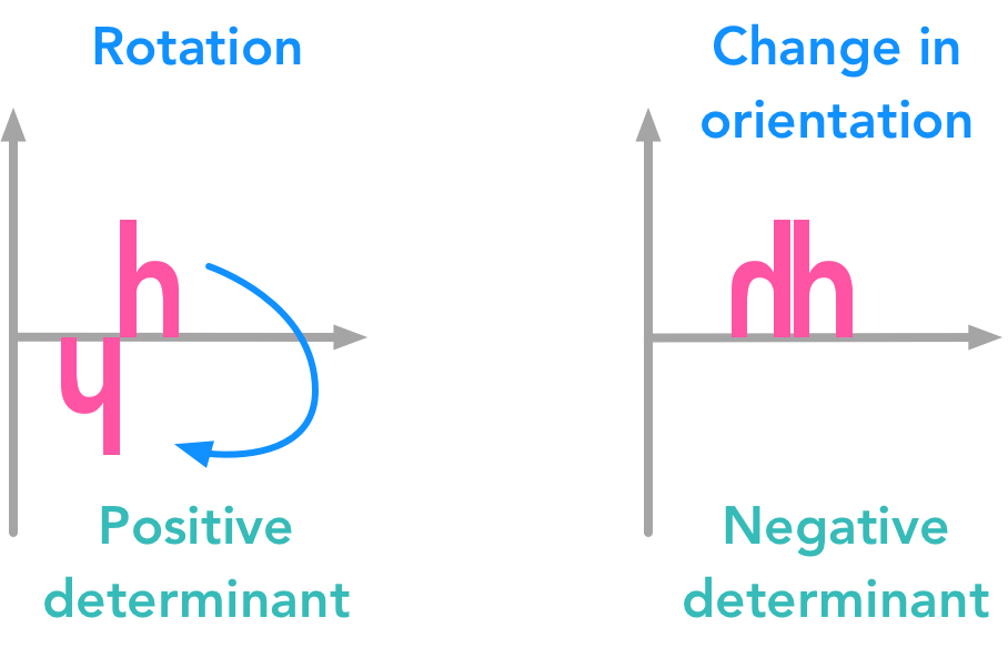The determinant of a matrix can tell you a lot of things about the transformation associated with this matrix

You can see that the second transformation can’t be obtained through rotation and rescaling. Thus the sign can tell you the nature of the transformation associated with the matrix!

In addition, the determinant also gives you the amount of transformation. If you take the n-dimensional unit cube and apply the matrix $\boldsymbol{A}$ on it, the absolute value of the determinant corresponds to the area of the transformed figure. You might believe me more easily after the following example.

Example 1.¶

To calculate the area of the shapes, we will use simple squares in 2 dimensions. The unit square area can be calculated with the Pythagorean theorem taking the two unit vectors.

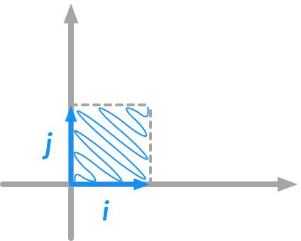The unit square area

The lengths of $i$ and $j$ are 1 thus the area of the unit square is 1.

Let’s start by creating both vectors in Python:

orange = '#FF9A13'
blue = '#1190FF'
    
i = [0, 1]
j = [1, 0]

plotVectors([i, j], [[blue], [orange]])
plt.xlim(-0.5, 3)
plt.ylim(-0.5, 3)
plt.show()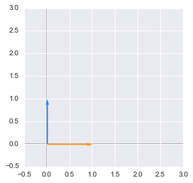

<matplotlib.figure.Figure at 0x109d78890>

We will apply

\boldsymbol{A}=\begin{bmatrix} 2 & 0\\\\ 0 & 2 \end{bmatrix}

(1)

to $i$ and $j$ . You can notice that this matrix is special: it is diagonal. So it will only rescale our space. No rotation here. More precisely, it will rescale each dimension the same way because the diagonal values are identical. Let’s create the matrix $\boldsymbol{A}$ :

A = np.array([[2, 0], [0, 2]])
A

array([[2, 0],
       [0, 2]])

Now we will apply $\boldsymbol{A}$ on our two unit vectors $i$ and $j$ and plot the resulting new vectors:

new_i = A.dot(i)
new_j = A.dot(j)
plotVectors([new_i, new_j], [['#1190FF'], ['#FF9A13']])
plt.xlim(-0.5, 3)
plt.ylim(-0.5, 3)
plt.show()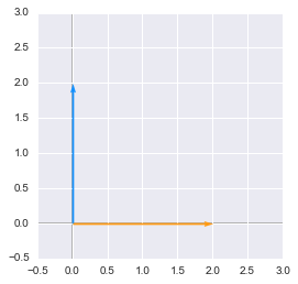

<matplotlib.figure.Figure at 0x109d164d0>

As expected, we can see that the square corresponding to $i$ and $j$ didn’t rotate but the lengths of $i$ and $j$ have doubled. We will now calculate the determinant of $\boldsymbol{A}$ (you can go to the Wikipedia article for more details about the calculation of the determinant):

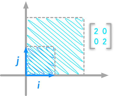Areas of the unit square and its transformation by the matrix

The unit square transformed by the matrix

np.linalg.det(A)

4.0

And yes, the transformation have multiplied the area of the unit square by 4. The lengths of $new_i$ and $new_j$ are 2 (thus $2\cdot2=4$ ).

Example 2.¶

Let’s see now an example of negative determinant.

We will transform the unit square with the matrix:

\boldsymbol{B}=\begin{bmatrix} -2 & 0\\\\ 0 & 2 \end{bmatrix}

(2)

Its determinant is -4:

B = np.array([[-2, 0], [0, 2]])
np.linalg.det(B)

-4.0

new_i_1 = B.dot(i)
new_j_1 = B.dot(j)
plotVectors([new_i_1, new_j_1], [['#1190FF'], ['#FF9A13']])
plt.xlim(-3, 0.5)
plt.ylim(-0.5, 3)
plt.show()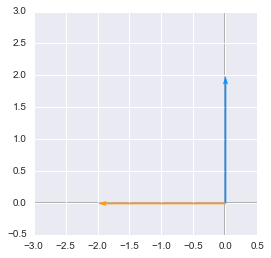

<matplotlib.figure.Figure at 0x109b16c10>

We can see that the matrices with determinant 2 and -2 modified the area of the unit square the same way.

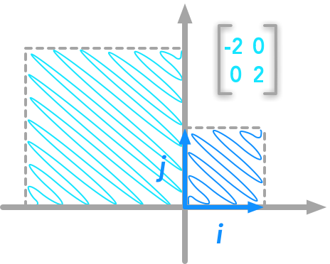Areas of the unit square and its transformation by the matrix with a negative determinant

The unit square transformed by the matrix with a negative determinant

The absolute value of the determinant shows that, as in the first example, the area of the new square is 4 times the area of the unit square. But this time, it was not just a rescaling but also a transformation. It is not obvious with only the unit vectors so let’s transform some random points. We will use the matrix

\boldsymbol{C}=\begin{bmatrix} -1 & 0\\\\ 0 & 1 \end{bmatrix}

(3)

that has a determinant equal to -1 for simplicity:

# Some random points
points = np.array([[1, 3], [2, 2], [3, 1], [4, 7], [5, 4]])

C = np.array([[-1, 0], [0, 1]])
np.linalg.det(C)

-1.0

Since the determinant is -1, the area of the space will not be changed. However, since it is negative we will observe a transformation that we can’t obtain through rotation:

newPoints = points.dot(C)

plt.figure()
plt.plot(points[:, 0], points[:, 1])
plt.plot(newPoints[:, 0], newPoints[:, 1])
plt.show()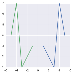

<matplotlib.figure.Figure at 0x108e64a90>

You can see that the transformation mirrored the initial shape.

Conclusion¶

We have seen that the determinant of a matrix is a special value telling us a lot of things on the transformation corresponding to this matrix. Now hang on and go to the last chapter on the Principal Component Analysis (PCA).

References¶

Linear transformations¶

Numpy¶

Numpy determinant