Giant Component and Phase Transition
Computer Science Dept, Ferdowsi University of Mashhad
In the previous page we counted edges, degrees and triangles in , and every answer was a number: the expected degree is , the degree distribution is Poisson, the number of triangles is roughly . This page asks a different kind of question — a geometric one. When we raise from 0 to 1, at which point does the graph stop being a dust of tiny components and grow one component that holds a positive fraction of all vertices?
The answer is a sharp change at , and the tool that explains it is the branching process. This is the cleanest example in the course of a threshold phenomenon: a quantity that is below a critical value and above it, with no gradual transition in between.
Goals
Read the component of a vertex as a branching process, with mean offspring .
Derive the survival probability from the fixed-point equation .
Locate the threshold and see why it is a rescaling, not a constant.
Simulate the largest component against and compare with the theory.
Know the second threshold, , where the graph becomes connected.
Meet the small-world model (Watts–Strogatz) as a one-paragraph survey.
1. The component of a vertex as a branching process
Fix a vertex and explore its component one vertex at a time. Vertex has neighbours, of mean . Take one of those neighbours; among the remaining vertices it expects new neighbours, and so on. As long as the explored set is small compared with , every newly discovered vertex contributes about new vertices, so the exploration is a Galton–Watson process with offspring distribution
The number of vertices in the component is the total progeny of this branching process. Two things follow at once:
If (subcritical) the expected offspring is below one, a generation dies out almost surely, and the component of has finite size with an exponential tail.
If (supercritical) there is a probability that the process never dies out; conditioned on survival it grows geometrically, that is, its size is .
The process is a good approximation only while the component is small; that is why it can say nothing about the giant component’s exact size. But the probability of survival is exactly what we need: it is the fraction of vertices that end up in the giant component.
2. The survival probability
Let be the probability that the process dies out starting from one vertex. A vertex dies out if each of its children dies out, so by the law of total probability, with ,
The equation always has the root . A second root in exists exactly when the derivative at 1, which is , exceeds one. Writing for the survival probability,
with for (the only root) and a unique positive root for . Expanding near gives
so the giant component grows linearly from zero with infinite slope — a second-order transition. In the graph itself the same quantity appears as the fraction of vertices in the giant component, which is the statement
in probability, for fixed and .
import numpy as np
import matplotlib.pyplot as plt
import networkx as nx
from scipy.sparse import coo_matrix
from scipy.sparse.csgraph import connected_components


def er_sizes(n, p, rng):
    '''Largest component size and number of components of G(n, p).

    Edges are sampled by drawing the binomial number of edges and then choosing
    their endpoints uniformly; for p = c/n the fraction of repeated pairs is
    O(1/n), which is negligible for the sizes we look at.
    '''
    m = rng.binomial(n * (n - 1) // 2, p)
    i = rng.integers(0, n, size=m)
    j = rng.integers(0, n, size=m)
    keep = i != j
    a = coo_matrix((np.ones(keep.sum()), (i[keep], j[keep])), shape=(n, n))
    ncomp, labels = connected_components(a, directed=False)
    return np.bincount(labels).max(), ncomp


def survival(c):
    '''Positive root of s = 1 - exp(-c s); zero for c <= 1 (bisection).'''
    if c <= 1:
        return 0.0
    lo, hi = 0.0, 1.0
    for _ in range(200):
        mid = 0.5 * (lo + hi)
        if mid - (1 - np.exp(-c * mid)) < 0:
            lo = mid
        else:
            hi = mid
    return 0.5 * (lo + hi)


cs = np.linspace(0.05, 3.0, 60)
theory = np.array([survival(c) for c in cs])

plt.plot(cs, theory, lw=2, label=r"$s=1-e^{-cs}$")
plt.axvline(1, c="k", ls=":", label=r"$c=1$ (critical)")
plt.axvspan(0, 1, color="0.9", zorder=0)
plt.xlabel(r"$c=np$")
plt.ylabel("surviving fraction $s$")
plt.title("Giant component: the fixed-point equation")
plt.legend()
plt.show()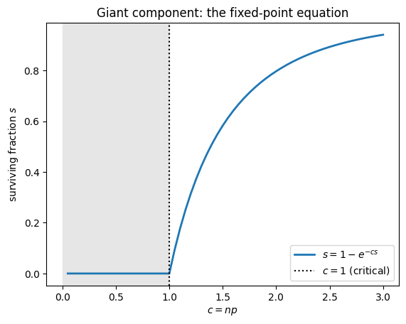
3. Why the threshold is and not a constant
The expectation of the degree is , so the question “is the mean degree above or below one?” is a question about the product , not about . Two consequences:
Scaling. keeps the mean degree fixed while grows. Any constant gives a graph that is a single dense blob — every vertex has neighbours — and the notion of “component” loses its interest. The interesting regime lives at scale .
Sharpness. The transition is not spread over an interval of of constant length: at the scale the largest component changes size, so the window has width in the number of edges, which is in . On the axis the transition looks sharp for large and blunt for small — exactly the finite-size effect we see in the next plot.
The same rescaling appears once more in this page: connectivity happens at , again times a slowly growing factor.
rng = np.random.default_rng(0)
grid = np.array([0.3, 0.5, 0.7, 0.85, 0.95, 1.0, 1.05, 1.15, 1.3, 1.5, 1.8, 2.2])
REPS = 8

fig, ax = plt.subplots(figsize=(7, 4.5))
ax.plot(cs, theory, "k--", lw=2, label="theory $s(c)$")

print(f"{'c':>5} {'s(c)':>7} " + " ".join(f"{'n=' + str(n):>8}" for n in (300, 1500, 6000)))
for c in grid:
    row = [np.mean([er_sizes(n, c / n, rng)[0] / n for _ in range(REPS)])
           for n in (300, 1500, 6000)]
    print(f"{c:5.2f} {survival(c):7.3f} " + " ".join(f"{v:8.3f}" for v in row))
    ax.plot([c], [row[-1]], "o", c="C2")

for n, colour in zip((300, 1500, 6000), ("C0", "C1", "C2")):
    mean = [np.mean([er_sizes(n, c / n, rng)[0] / n for _ in range(REPS)]) for c in grid]
    ax.plot(grid, mean, "o-", c=colour, label=f"$n={n}$")

ax.axvline(1, c="k", ls=":", lw=1)
ax.set_xlabel(r"$c=np$")
ax.set_ylabel(r"$|C_{\max}|/n$")
ax.set_title("Largest component against the mean degree")
ax.legend()
plt.show()
c s(c) n=300 n=1500 n=6000
0.30 0.000 0.022 0.005 0.002
0.50 0.000 0.025 0.009 0.003
0.70 0.000 0.041 0.021 0.005
0.85 0.000 0.062 0.028 0.011
0.95 0.000 0.155 0.072 0.030
1.00 0.000 0.176 0.077 0.052
1.05 0.094 0.166 0.162 0.100
1.15 0.249 0.299 0.256 0.250
1.30 0.423 0.375 0.419 0.420
1.50 0.583 0.541 0.564 0.584
1.80 0.732 0.711 0.725 0.730
2.20 0.844 0.829 0.837 0.842
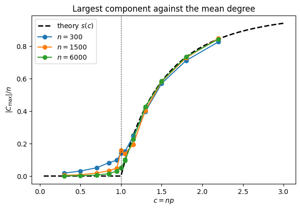
Small rounds the corner of the curve and pushes the apparent threshold to the right: for the giant component only clearly appears around , while the limiting curve turns at . This is the finite-size window of the previous section, not a disagreement with the theory. Note also that close to eight repetitions are not enough: half of the runs have a giant component and half do not, so the average jumps around. That is the bimodality of the next plot, seen from the outside.
A sharper diagnostic than the mean is the distribution of at a fixed near 1. Below the threshold it is small and concentrated; above it, a fraction of the runs produce a giant component while the rest stay small, so the histogram is bimodal right at the transition.
n = 2000
fig, axes = plt.subplots(1, 3, figsize=(11, 3.2), sharey=True)
for ax, c in zip(axes, (0.95, 1.0, 1.05)):
    fracs = [er_sizes(n, c / n, rng)[0] / n for _ in range(40)]
    ax.hist(fracs, bins=12, color="steelblue")
    ax.set_title(f"$c={c}$")
    ax.set_xlabel(r"$|C_{\max}|/n$")
axes[0].set_ylabel("runs")
fig.suptitle("Bimodality at the critical point ($n=2000$, 40 runs each)", y=1.03)
plt.show()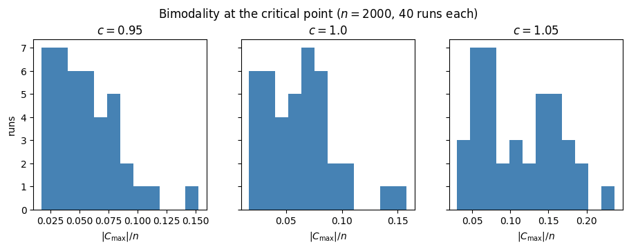
4. The second threshold: connectivity
A graph can have a giant component and still be disconnected: one isolated vertex is enough. The component of a fixed vertex has size only if the branching process stays alive and reaches every one of the remaining vertices; the latter costs about generations, and the resulting threshold is
The reason the extra factor is logarithmic is the coupon-collector argument: the last isolated vertex is found by a union bound over vertices, each isolated with probability , and requires . So the graph becomes connected a constant factor above the point where the giant component appears.
n = 400
ts = np.linspace(0.4, 2.0, 9)
connected = [np.mean([er_sizes(n, t * np.log(n) / n, rng)[1] == 1 for _ in range(20)]) for t in ts]

plt.plot(ts, connected, "o-")
plt.axvline(1, c="k", ls=":", label=r"$p=\log n/n$")
plt.xlabel(r"$t$ in $p = t\log n/n$")
plt.ylabel("fraction of runs that are connected")
plt.title(f"Connectivity threshold, $n={n}$")
plt.legend()
plt.show()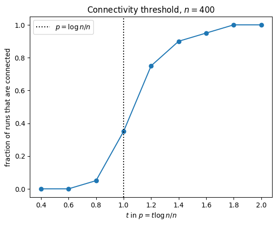
5. Small world: one paragraph
Erdős–Rényi graphs have short paths (diameter ) but almost no triangles. Real networks — social, biological, citation — have both. Watts and Strogatz start from a ring where each vertex is joined to its nearest neighbours, so clustering is high and paths are long, and then rewire each edge with probability to a uniformly random vertex. A tiny destroys the long paths (a few shortcuts are enough) while leaving most local triangles intact: the small-world regime. The model is here only as a bridge — clustering coefficients, path lengths and the degree distributions of real networks belong to a graph-mining course.
betas = [0.0, 0.01, 0.03, 0.1, 0.3, 1.0]
paths, clustering = [], []
for b in betas:
    g = nx.watts_strogatz_graph(300, 6, b, seed=1)
    paths.append(nx.average_shortest_path_length(g))
    clustering.append(nx.average_clustering(g))

fig, ax1 = plt.subplots(figsize=(6.5, 4))
ax1.semilogx(np.maximum(betas, 1e-3), paths, "o-", c="C0")
ax1.set_xlabel(r"rewiring probability $\beta$ (0 drawn at $10^{-3}$)")
ax1.set_ylabel("average shortest path", c="C0")

ax2 = ax1.twinx()
ax2.semilogx(np.maximum(betas, 1e-3), clustering, "s--", c="C1")
ax2.set_ylabel("average clustering", c="C1")
ax1.set_title(r"Watts–Strogatz, $n=300$, $k=6$")
plt.show()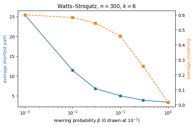
6. What to remember
The component of a vertex is a branching process with mean offspring ; the giant component exists iff , that is iff .
Its asymptotic size is the survival probability , the positive root of , which behaves like near the threshold.
Two different thresholds live at the same scale : the giant component at and connectivity at .
The tree-like approximation behind the branching process is what fails for the size, not for the threshold: loops are rare exactly when .
The next page uses a graph as a state space rather than as a random object: a random walk on a fixed graph, its stationary distribution, and PageRank.
Exercises
Model the component of a vertex as a branching process with Poisson offspring of mean . Show that the survival probability is zero for and solve for .
Simulate for with around , plot the size of the largest component against , and locate the transition.
Explain why the threshold is and not a constant: rescale by and say which quantity stays fixed.
Show that the expected number of triangles is and that it tends to a constant when . Explain why the branching-process approximation of the component is exact in this regime (hint: count cycles).
Let be the extinction probability. Prove that is always a root of , and that the equation has a second root in if and only if , by looking at the derivative of at .
Use the coupon-collector argument to show that makes the probability of an isolated vertex tend to zero, and that leaves isolated vertices on average.
In the Watts–Strogatz experiment above, explain why the clustering coefficient barely changes for while the average path length already collapses. Which of the two is a local quantity?
Sources
Blum, Hopcroft, Kannan, Foundations of Data Science, Ch. 7–8 (branching processes and the giant component).
Durrett, Random Graph Dynamics, Ch. 1–2 (the critical window and the scale).
Watts, D. and Strogatz, S., “Collective dynamics of ‘small-world’ networks”, Nature 393, 1998.
Bollobás, Random Graphs, Ch. 5–7 (connectivity and the threshold).