Erdős–Rényi Random Graphs
So far a graph was a single object: an adjacency matrix, a degree sequence, a set of edges. The Erdős–Rényi model replaces that object by a probability distribution over graphs. We can then ask questions such as “how many edges does a typical graph have?” or “when does a giant connected component appear?”, and answer them exactly — and check the answers by simulation.
Reading. Blum, Hopcroft & Kannan, Foundations of Data Science, Ch. 4; van Steen, Graph Theory and Complex Networks, Ch. 3.
Why model graphs randomly?
Null model. What does a network look like when there is no structure at all? Anything that the random model does not produce (heavy-tailed degrees, many triangles, small diameter) is what we mean by “structure” in real data.
Generative model. Statements such as “most graphs are connected” hold with high probability (whp) — for a single graph they are simply true or false.
Testbed. Community detection, spectral clustering or PageRank are first tested on random graphs, where the correct answer is known by construction.
%matplotlib inline
import math
from collections import Counter

import matplotlib.pyplot as plt
import networkx as nx
import numpy as np

plt.rcParams["figure.figsize"] = (6, 4)
rng = np.random.default_rng(7)
The two models
Definition (Erdős–Rényi, ). Fix vertices. For each of the unordered pairs, insert the edge independently with probability .
Definition (). All graphs with vertices and exactly edges are equally likely.
The two are closely related: is conditioned on having exactly edges (with ), and for large the conditioning changes almost nothing.
n, p = 200, 0.05
G1 = nx.gnp_random_graph(n, p, seed=1)          # G(n, p)
G2 = nx.gnm_random_graph(n, nx.gnp_random_graph(n, p, seed=2).number_of_edges(), seed=3)  # G(n, m)

print("n =", n, " p =", p, " number of possible pairs =", math.comb(n, 2))
print("G(n,p) edges:", G1.number_of_edges(), "   G(n,m) edges:", G2.number_of_edges())
n = 200 p = 0.05 number of possible pairs = 19900
G(n,p) edges: 1025 G(n,m) edges: 996
Number of edges
Let . The number of edges is a sum of independent Bernoulli variables, hence
The mean degree follows immediately: .
n, p, reps = 500, 0.05, 2000
N = math.comb(n, 2)

counts = np.array([nx.gnp_random_graph(n, p, seed=s).number_of_edges() for s in range(reps)])

print(f"theory : mean = {N*p:.1f}   std = {math.sqrt(N*p*(1-p)):.2f}")
print(f"empirical: mean = {counts.mean():.1f}   std = {counts.std():.2f}")
theory : mean = 6237.5 std = 76.98
empirical: mean = 6239.1 std = 77.34
The degree distribution
The degree of one fixed vertex is the number of successes among the pairs that contain it:
Poisson limit
The interesting regime is a constant average degree : take and let . Then and
(The first factor behaves like , the last one like .) So a large sparse Erdős–Rényi graph has Poisson degrees: most vertices have degree close to , and the maximum degree is only . Real networks look very different — see the last section.
n, c = 2000, 3
p = c / (n - 1)
G = nx.gnp_random_graph(n, p, seed=11)

degrees = np.array([d for _, d in G.degree()])
k = np.arange(0, degrees.max() + 1)

binomial = [math.comb(n - 1, int(i)) * p**i * (1 - p) ** (n - 1 - i) for i in k]
poisson = [math.exp(-c) * c**i / math.factorial(int(i)) for i in k]

plt.bar(k, np.bincount(degrees, minlength=len(k)) / n, width=0.8,
        label="empirical", color="0.8", edgecolor="0.5")
plt.plot(k, binomial, "o-", ms=4, label=r"$\mathrm{Bin}(n-1,p)$")
plt.plot(k, poisson, "s--", ms=4, label=r"$\mathrm{Poisson}(c),\ c=3$")
plt.xlabel("degree $k$")
plt.ylabel("fraction of vertices")
plt.title(f"Degree distribution, $G(n,p)$ with $n={n}$, $c=(n-1)p=3$")
plt.legend()
plt.show()

print("mean degree: empirical =", degrees.mean().round(3), " theory c =", c)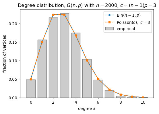
mean degree: empirical = 2.961 theory c = 3
Triangles and clustering
For a fixed triple of vertices to form a triangle, its three edges must be present:
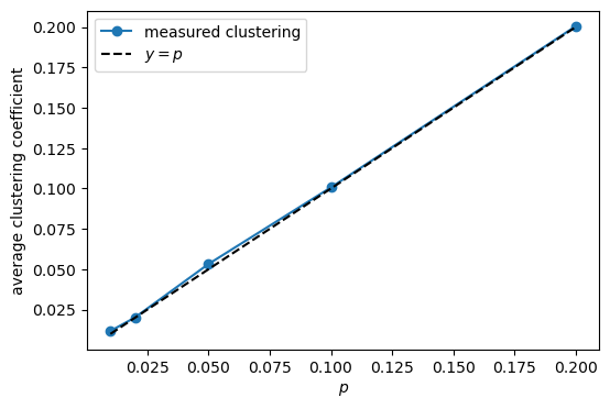
The local clustering coefficient of a vertex is the fraction of pairs of its neighbours that are themselves connected. In those edges are independent of the neighbourhood, so on average
which is tiny for the sparse graphs we care about (). This is the main defect of the model: real social networks have clustering coefficients of order 10-1 while is of order 10-3.
n = 400
ps = np.array([0.01, 0.02, 0.05, 0.1, 0.2])
clustering, expected_triangles, measured_triangles = [], [], []

for p in ps:
    G = nx.gnp_random_graph(n, p, seed=21)
    clustering.append(nx.average_clustering(G))
    expected_triangles.append(math.comb(n, 3) * p**3)
    measured_triangles.append(sum(nx.triangles(G).values()) // 3)

for p, cl, eT, mT in zip(ps, clustering, expected_triangles, measured_triangles):
    print(f"p = {p:5.2f} | avg clustering = {cl:.4f} (p = {p:.4f}) | triangles: measured {mT:6d}, theory {eT:9.1f}")

plt.plot(ps, clustering, "o-", label="measured clustering")
plt.plot(ps, ps, "k--", label=r"$y=p$")
plt.xlabel("$p$")
plt.ylabel("average clustering coefficient")
plt.legend()
plt.show()
p = 0.01 | avg clustering = 0.0118 (p = 0.0100) | triangles: measured 11, theory 10.6
p = 0.02 | avg clustering = 0.0202 (p = 0.0200) | triangles: measured 82, theory 84.7
p = 0.05 | avg clustering = 0.0532 (p = 0.0500) | triangles: measured 1359, theory 1323.4
p = 0.10 | avg clustering = 0.1007 (p = 0.1000) | triangles: measured 10785, theory 10586.8
p = 0.20 | avg clustering = 0.2005 (p = 0.2000) | triangles: measured 84181, theory 84694.4
Thresholds: the graph changes qualitatively as grows
Most statements about are threshold statements: there is a value such that below it a property holds whp, and above it fails whp (or vice versa).
| Property | Threshold | Typical picture |
|---|---|---|
| at least one edge | isolated edges | |
| a fixed subgraph with vertices, edges | e.g. triangles at | |
| a tree on vertices | e.g. paths of length 2 at | |
| giant component | mean degree | |
| connectivity | every vertex has a neighbour |
The last two are the ones we care about. Both are read off the number of isolated vertices: for ,
which tends to 0 when and to when — hence the threshold .
n = 500
cs = [0.6, 0.8, 1.0, 1.2, 1.5]
print(f"{'c':>5} {'p':>10} {'isolated (measured)':>20} {'n^(1-c)':>10}")
for c in cs:
    p = c * math.log(n) / n
    G = nx.gnp_random_graph(n, p, seed=int(100 * c))
    isolated = sum(1 for _, d in G.degree() if d == 0)
    print(f"{c:5.2f} {p:10.6f} {isolated:20d} {n ** (1 - c):10.2f}")
c p isolated (measured) n^(1-c)
0.60 0.007458 18 12.01
0.80 0.009943 1 3.47
1.00 0.012429 3 1.00
1.20 0.014915 0 0.29
1.50 0.018644 0 0.04
The giant component (a preview)
Take and let be the fraction of vertices in the largest component. A branching-process argument (each neighbour has on average further neighbours) gives the self-consistency equation
whose non-zero solution exists exactly when . This is the phase transition: for all components are of size , for a positive fraction of the vertices sits in one component. The next page derives this in detail; here we only check it experimentally.
def giant_fraction_theory(c):
    """Solve S = 1 - exp(-c S) by fixed-point iteration (S = 0 is always a solution)."""
    if c <= 1:
        return 0.0
    S = 0.5
    for _ in range(200):
        S = 1 - math.exp(-c * S)
    return S


n = 2000
cs = np.linspace(0.5, 3.0, 11)
measured = []
for c in cs:
    G = nx.gnp_random_graph(n, c / n, seed=int(1000 * c))
    largest = max(len(comp) for comp in nx.connected_components(G))
    measured.append(largest / n)

plt.plot(cs, [giant_fraction_theory(c) for c in cs], "-", label=r"$S = 1-e^{-cS}$")
plt.plot(cs, measured, "o", label=f"simulation, $n={n}$")
plt.axvline(1.0, color="0.6", ls=":", label="critical mean degree $c=1$")
plt.xlabel("mean degree $c = (n-1)p$")
plt.ylabel("size of largest component / $n$")
plt.legend()
plt.show()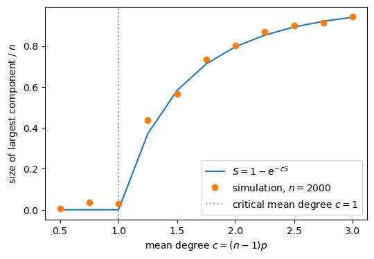
Lab: what a random graph looks like
Keeping fixed and varying the mean degree shows the three regimes: a dust of tiny components, a critical graph, and a graph dominated by one giant component.
n = 60
fig, axes = plt.subplots(2, 3, figsize=(12, 7))
for ax, c in zip(axes.ravel(), [0.5, 1.0, 2.0, 4.0, 8.0, 16.0]):
    G = nx.gnp_random_graph(n, c / (n - 1), seed=int(10 * c) + 5)
    largest = max(len(comp) for comp in nx.connected_components(G))
    nx.draw(G, ax=ax, node_size=25, width=0.6, node_color="#4c78a8", edge_color="0.7")
    ax.set_title(f"$c={c:g}$  |  edges {G.number_of_edges()}, largest {largest}/{n}", fontsize=10)
plt.tight_layout()
plt.show()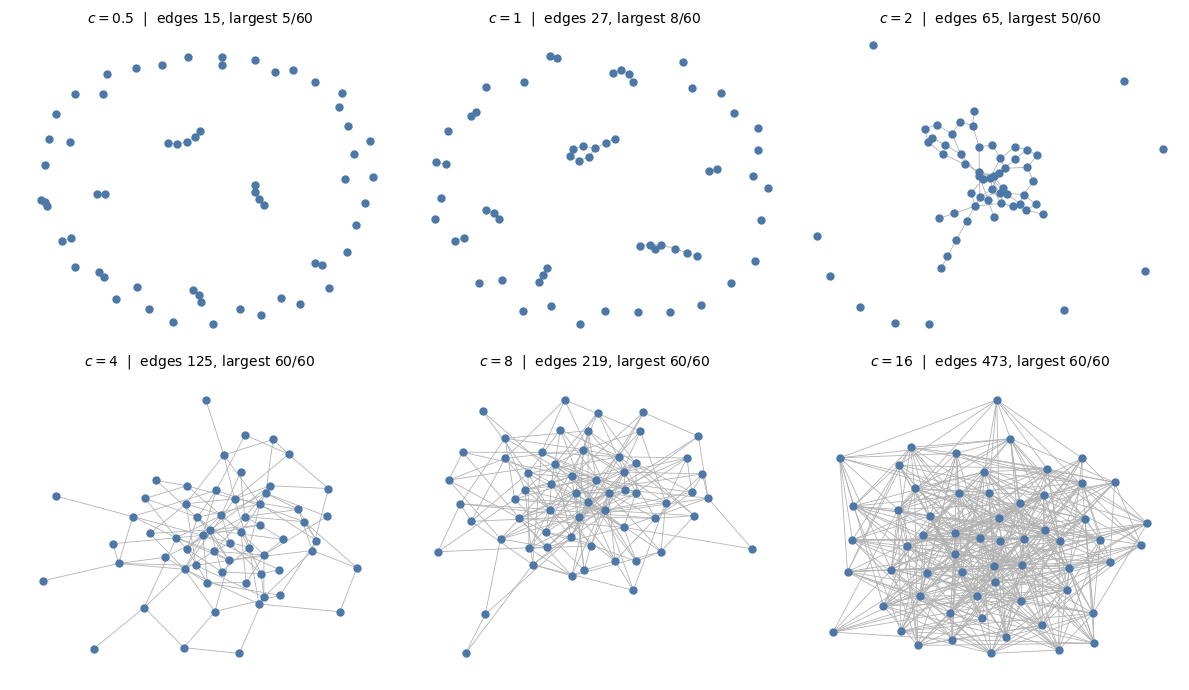
What the model does not do
A single parameter cannot describe a real network. Three systematic mismatches motivate the models that come next in this course:
Degrees. has Poisson degrees; web graphs, citations and social networks have heavy-tailed (power-law) degrees — a few hubs carry a large fraction of the edges.
Clustering. Triangles are rare (); in real social networks your friends are friends much more often than chance would predict. The configuration model (random graph with a prescribed degree sequence) and the Watts–Strogatz small-world model are the two standard repairs.
Geometry. Distance in is — very small, but the graph has no notion of “close” nodes, which real data (images, cities, the web) usually have.
Still, the Erdős–Rényi graph is the reference point against which all of these are measured.
Exercises
Derive and for , and use Chebyshev’s inequality to show that in probability.
Show that for the number of isolated vertices converges in distribution to scaled by , and deduce the connectivity threshold .
For fixed , compute the expected number of -cliques and conclude that -cliques appear around .
Generate and compare its degree distribution with at ; explain the small difference you observe.
For , find empirically the smallest at which the graph is connected, and compare with . Reproduce the table of thresholds above.
Optional. Repeat the giant-component experiment for the configuration model with a power-law degree sequence and describe how the transition changes.
References
P. Erdős and A. Rényi, On the evolution of random graphs, Publ. Math. Inst. Hung. Acad. Sci. 5 (1960), 17–61.
A. Blum, J. Hopcroft and R. Kannan, Foundations of Data Science, Cambridge University Press, Ch. 4 (Random Graphs).
M. van Steen, Graph Theory and Complex Networks: An Introduction, Ch. 3.
NetworkX documentation:
gnp_random_graph,gnm_random_graph,connected_components.