Clustering Validation
Mahmood Amintoosi, Fall 2026
Computer Science Dept, Ferdowsi University of Mashhad
This page follows chapter 17 of Zaki & Meira (2020), Clustering Validation.
Source
import numpy as np
import matplotlib.pyplot as plt
plt.rcParams['figure.dpi'] = 120
Introduction to Clustering Validation
Clustering validation assesses the quality of a clustering. Every algorithm returns some partition of the data; the question is whether that partition is any good, and how two candidate partitions can be compared. The measures fall into three families:
External measures: use external information, the ground-truth labels.
Internal measures: use only the data and the clustering result.
Relative measures: compare two clusterings of the same data with each other, without any ground truth.
Learning objectives. By the end you should be able to
build the contingency table of a clustering against the ground truth, and read it;
compute and interpret purity, precision/recall/F, maximum matching, Jaccard, Rand and ARI, and say what each one ignores;
explain why accuracy cannot be used on cluster labels;
use internal measures (silhouette, SSE) and say why none of them identifies the “true” number of clusters;
choose on the SSE curve with the elbow rule, and read the maximum-matching score as an assignment problem;
find the measures that did not fit on this page — NMI, the gap statistic and the assignment problem in full — in the appendix.
Notation
Zaki writes for the number of clusters and for the number of ground-truth classes. This page keeps those letters, so that the formulas match the book; note that the k-means pages of this course use for the number of clusters. In every formula below counts the points of cluster that belong to class , and is the number of points.
External Measures
External measures assume that the correct or ground-truth clustering is known a priori, which is used to evaluate a given clustering.
Let be a dataset consisting of points in a -dimensional space, partitioned into clusters. Let denote the ground-truth cluster membership or label information for each point.
The ground-truth clustering is given as:
where the cluster consists of all the points with label , i.e.,
We refer to as the ground-truth partitioning, and to each as a partition (class).
Let denote a clustering of the same dataset into clusters, obtained via some clustering algorithm, and let denote the cluster label for .
External evaluation measures try to capture the extent to which points from the same partition appear in the same cluster, and the extent to which points from different partitions are grouped in different clusters.
All of the external measures rely on the contingency table that is induced by a clustering and the ground-truth partitioning , defined as follows:
The count denotes the number of points that are common to cluster and ground-truth partition .
Let denote the number of points in cluster , and let denote the number of points in partition . The contingency table can be computed from and in time by examining the partition and cluster labels, and , for each point and incrementing the corresponding count — the first index is the cluster label, the second the class label, so that rows of are clusters and columns are classes.
Source
import pandas as pd

def display_contingency_table_pandas(table, class_names=None, cluster_names=None):
    r, k = table.shape
    if class_names is None:
        class_names = [f"Class {j}" for j in range(k)]
    if cluster_names is None:
        subscript = "₀₁₂₃₄₅₆₇₈₉"
        cluster_names = [f"C{subscript[i]}" for i in range(r)]

    df = pd.DataFrame(table, index=cluster_names, columns=class_names)
    display(df.style
              .set_properties(**{'text-align': 'center'})
              .set_table_styles([
                  {'selector': 'th',
                   'props': [('text-align', 'center'),
                             ('background-color', '#f2f2f2'),
                             ('border', '1px solid #ccc')]},
                  {'selector': 'td',
                   'props': [('border', '1px solid #ccc')]},
              ]))
import numpy as np
def compute_contingency_table(cluster_labels, true_labels):
"""Contingency table of a clustering against the ground truth.
Returns an ``(r, k)`` integer matrix: rows index clusters, columns index classes,
so ``table[i, j]`` is the number of points of cluster ``i`` in class ``j``.
"""
unique_classes, class_map = np.unique(true_labels, return_inverse=True)
unique_clusters, cluster_map = np.unique(cluster_labels, return_inverse=True)
table = np.zeros((len(unique_clusters), len(unique_classes)), dtype=int)
np.add.at(table, (cluster_map, class_map), 1)
return tableA first reference point: a perfect clustering
Before looking at anything that goes wrong, we need a baseline. The table below is obtained when every cluster matches exactly one ground-truth class. The contingency matrix is diagonal: every off-diagonal entry is zero.
This is the only case in which the “ideal” value of any reasonable external measure is reached (1 for purity and ARI). Every other example on this page should be compared against this baseline.
# Example A — perfect clustering
true_labels    = np.array([0, 0, 0, 1, 1, 1, 2, 2, 2])
cluster_labels = np.array([0, 0, 0, 1, 1, 1, 2, 2, 2])

table = compute_contingency_table(cluster_labels, true_labels)
display_contingency_table_pandas(table)A good clustering with a small, symmetric mistake
Most realistic clusterings are almost right. Here, C₀ is still perfectly
pure, but C₁ and C₂ have swapped one point each: one point from class
T₁ landed in C₂ and one from T₂ landed in C₁.
The table is almost diagonal, so purity and ARI will both be close to but slightly below 1. This is the typical “slightly imperfect” case that most practical algorithms produce.
# Example B — almost perfect, one swap
true_labels    = np.array([0, 0, 0, 1, 1, 1, 2, 2, 2])
cluster_labels = np.array([0, 0, 0, 1, 1, 2, 2, 2, 1])

table = compute_contingency_table(cluster_labels, true_labels)
display_contingency_table_pandas(table)Cluster ids are arbitrary labels, not orderings
The partition below is exactly the same as the one in Example B; only the
ids of the clusters have been permuted. C₁ in this example is what C₂ was
before, and vice versa.
The table is the same as B with its rows rearranged — and every external
measure gives the same numerical value. This is the reason all external
measures must be invariant to permutations of the cluster ids: the numbers
0, 1, 2 returned by KMeans.labels_ are just names, not a ranking.
# Example C — same partition as B, cluster ids relabelled
true_labels    = np.array([0, 0, 0, 1, 1, 1, 2, 2, 2])
cluster_labels = np.array([1, 1, 1, 2, 2, 0, 0, 0, 2])

table = compute_contingency_table(cluster_labels, true_labels)
display_contingency_table_pandas(table)A weak clustering with symmetric spread
Now the clustering is not close to the ground truth at all. Every cluster contains points from two different classes, and every class is split across two clusters. The table has several non-zero entries per row and per column, but no row or column is “pure”.
Purity will be around 0.5, ARI will be clearly below 1. Notice that there is still some signal: the diagonal entries are not zero, so the clustering is not random — it is simply weak.
# Example D — weak clustering, scattered table
true_labels    = np.array([0, 0, 1, 1, 2, 2])
cluster_labels = np.array([0, 1, 1, 2, 2, 0])

table = compute_contingency_table(cluster_labels, true_labels)
display_contingency_table_pandas(table)A deceptive case: a perfectly uniform table
This example has a contingency table in which every entry is exactly equal. Every cluster contains one point from each class, and every class is spread evenly across all clusters.
This is the most instructive case on the page. The table looks neat and regular, yet it carries no information: knowing which cluster a point was assigned to tells us nothing about its true class.
Purity is exactly 1/3, and ARI is exactly 0 — the same values a
completely random assignment would produce. Regularity of the table is not the
same thing as usefulness of the clustering.
# Example E — deceptive, uniform contingency table
true_labels    = np.array([0, 0, 0, 1, 1, 1, 2, 2, 2])
cluster_labels = np.array([0, 1, 2, 1, 2, 0, 2, 0, 1])

table = compute_contingency_table(cluster_labels, true_labels)
display_contingency_table_pandas(table)When the number of clusters differs from the number of classes
All examples so far had : as many clusters as ground-truth classes.
But K-means is run with a fixed K that the user chooses, and there is no
guarantee that K matches the number of true classes.
In the example below, the ground truth has three classes but the algorithm produced four clusters — it has over-segmented one of the classes into two pieces. The contingency table is therefore not square, and no simple “accuracy” can be computed: there is no one-to-one correspondence between cluster ids and class ids.
Purity is still computable and still meaningful: it asks, for each cluster,
how pure it is, and then averages. But an over-segmented clustering gets a
suspiciously high purity, because small pure clusters are easy to form. ARI
penalises this properly, which is exactly why it is preferred in practice when K
is not known in advance.
# Example F — k = 4 clusters vs r = 3 classes (over-segmentation)
# The 3 points of class T₀ are split across two clusters: C₀ and C₃.
true_labels    = np.array([0, 0, 0, 1, 1, 1, 2, 2, 2])
cluster_labels = np.array([0, 0, 3, 1, 1, 1, 2, 2, 2])

table = compute_contingency_table(cluster_labels, true_labels)
display_contingency_table_pandas(table)The opposite case: too few clusters
Here the situation is reversed: the algorithm was run with , but there are three true classes. Two of them have been merged into a single cluster.
The contingency table is now a matrix, with one row containing points from two different classes. Purity drops immediately, because that row has two non-zero entries of comparable size. Under-segmentation is much harder to hide than over-segmentation.
# Example G — k = 2 clusters vs r = 3 classes (under-segmentation)
# Classes T₀ and T₁ have been merged into a single cluster C₀.
true_labels    = np.array([0, 0, 0, 1, 1, 1, 2, 2, 2])
cluster_labels = np.array([0, 0, 0, 0, 0, 0, 1, 1, 1])

table = compute_contingency_table(cluster_labels, true_labels)
display_contingency_table_pandas(table)Efficient Contingency Table Computation with np.add.at
When implementing clustering validation metrics, constructing a contingency table is a key step. One efficient way to do this in NumPy is using np.add.at. This method ensures correct accumulation of counts when duplicate indices are present.
Why np.add.at?
Unlike simple indexed incrementation, such as:
contingency_table[cluster_map, class_map] += 1NumPy’s fancy indexing creates a temporary copy, meaning updates to repeated indices may not accumulate correctly. Instead, np.add.at ensures in-place modifications:
np.add.at(contingency_table, (cluster_map, class_map), 1)Example: Difference Between Direct Indexing and np.add.at
Here’s an example illustrating how np.add.at correctly handles duplicate indices while direct indexing may fail:
import numpy as np

def compute_contingency_table_direct(cluster_labels, true_labels):
    """Same table, built with direct indexed incrementation."""
    unique_classes, class_map = np.unique(true_labels, return_inverse=True)
    unique_clusters, cluster_map = np.unique(cluster_labels, return_inverse=True)

    table = np.zeros((len(unique_clusters), len(unique_classes)), dtype=int)
    table[cluster_map, class_map] += 1  # a temporary copy is written back: duplicates are lost
    return table
import numpy as np
true_labels = np.array([0, 0, 1, 1, 1, 2, 2, 2, 2])
cluster_labels = np.array([0, 1, 1, 1, 1, 2, 2, 2, 2])
contingency_table_at = compute_contingency_table(cluster_labels, true_labels)
contingency_table_direct = compute_contingency_table_direct(cluster_labels, true_labels)
print("Using direct indexing:")
display_contingency_table_pandas(contingency_table_direct)
print("\nUsing np.add.at:")
display_contingency_table_pandas(contingency_table_at)Using direct indexing:
Using np.add.at:
1. Purity
Purity measures how “pure” each cluster is by the fraction of points from the majority class:
Where:
= total number of points
= number of clusters
= number of true classes
= number of points in cluster from class
def purity_score(cluster_labels, true_labels):
    contingency_matrix = compute_contingency_table(cluster_labels, true_labels)
    return np.sum(np.amax(contingency_matrix, axis=1)) / np.sum(contingency_matrix)
Let’s consider an example where we achieve high purity, ensuring our clustering is well-aligned with the ground-truth partitioning.
Example Data
Suppose we have the following clustering and ground-truth labels:
true_labels    = np.array([0, 0, 1, 1, 1, 2])
cluster_labels = np.array([0, 0, 1, 1, 2, 2])
Here, each cluster aligns better with a single true class.
Compute Contingency Table
Using the compute_contingency_table function, we obtain:
| Class 0 | Class 1 | Class 2 | |
|---|---|---|---|
| C₀ | 2 | 0 | 0 |
| C₁ | 0 | 2 | 0 |
| C₂ | 0 | 1 | 1 |
Middle Computations
Step 1: Find the max of each row:
max(C₀) = 2max(C₁) = 2max(C₂) = 1
Step 2: Sum the max values:
Step 3: Compute purity:
true_labels = np.array([0, 0, 1, 1, 1, 2])
cluster_labels = np.array([0, 0, 1, 1, 2, 2])

score = purity_score(cluster_labels, true_labels)
print(f"Purity Score: {score:.3f}")  # Expected output: 0.833
Purity Score: 0.833
purity is invariant to cluster labels, meaning that relabeling clusters doesn’t change the score as long as the assignment itself remains consistent.
Let’s take the previous clustering but shift the cluster labels (e.g., renaming clusters C₀ C₂, C₁ C₀, C₂ C₁):
import numpy as np

# Original clustering labels
true_labels            = np.array([0, 0, 1, 1, 1, 2])
cluster_labels         = np.array([0, 0, 1, 1, 2, 2])
shifted_cluster_labels = np.array([2, 2, 0, 0, 1, 1]) # Shifted cluster labels (mapping: 0 → 2, 1 → 0, 2 → 1)

# Compute purity scores for both cases
original_purity = purity_score(cluster_labels, true_labels)
shifted_purity = purity_score(shifted_cluster_labels, true_labels)

print(f"Original Purity: {original_purity:.3f}")  # Expected output: 0.833
print(f"Shifted Labels Purity: {shifted_purity:.3f}")  # Expected output: 0.833 (same!)
Original Purity: 0.833
Shifted Labels Purity: 0.833
Why Does Purity Stay the Same?
The mapping between clusters and ground-truth partitions hasn’t changed, only their labels.
Since purity only depends on how well clusters match ground-truth partitions, renaming clusters doesn’t affect purity calculations.
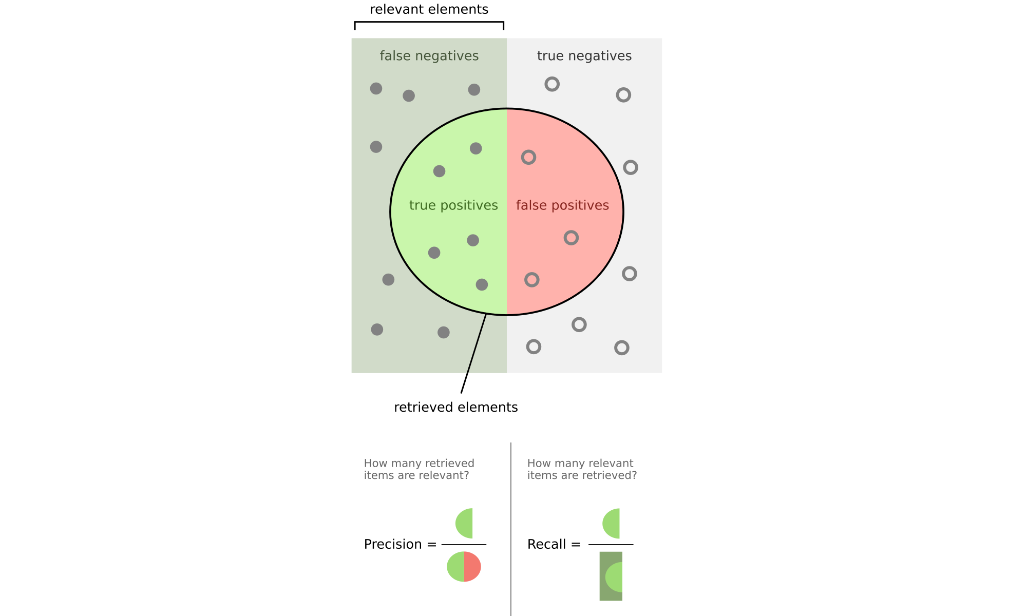
2. Precision, Recall and F-measure
For each cluster :
Precision: Fraction of points in cluster from majority class
Recall: Fraction of points from class found in cluster
Precision
Given cluster , let denote the partition that contains the maximum number of points from ,
that is, the index of the largest entry in row of the contingency table. The precision of a cluster is the same as its purity:
Recall
The recall of cluster is defined as:
where .
F-Measure
The F-measure is the harmonic mean of the precision and recall values for each :
The F-measure for the clustering is the mean of clusterwise F-measure values:
3. Maximum Matching
Finds the best matching between clusters and true classes to maximize overlap:
Where is a matching between clusters and classes.
Maximum weight matching (following Zaki & Meira (2020))
Let be a bipartite graph over the vertex set , and let the edge set be with edge weights . A matching in is a subset of , such that the edges in are pairwise nonadjacent, meaning they do not have a common vertex.
The maximum weight matching in is given as:
where is the sum of all edge weights in matching , given as .
Maximum Matching Examples (Bipartite Graph Interpretation)
Example 1 — Over-segmentation: one cluster is left unmatched
Scenario. Ten fruits with three true classes. The algorithm has split the apples into two clusters () and merged oranges and bananas into a single cluster ().
True Categories (T₁ = apples, T₂ = oranges, T₃ = bananas):
T₁: apple1, apple2, apple3, apple4, apple5      (5 apples)
T₂: orange1, orange2, orange3                    (3 oranges)
T₃: banana1, banana2                             (2 bananas)

Cluster Assignments (C₁, C₂, C₃):
C₁: [apple1, apple2, apple3]                     → 3 apples
C₂: [apple4, apple5]                             → 2 apples       ← over-segmentation
C₃: [orange1, orange2, orange3, banana1, banana2] → 3 oranges, 2 bananas
Contingency table
| Apples () | Oranges () | Bananas () | ||
|---|---|---|---|---|
| 3 | 0 | 0 | 3 | |
| 2 | 0 | 0 | 2 | |
| 0 | 3 | 2 | 5 | |
| 5 | 3 | 2 | 10 |
Purity is optimistic
Purity sees three “pure” clusters and reports a high value, even though both and claim the apple class at the same time. The one-to-one constraint that a classifier would impose is invisible to Purity.
Maximum Matching sees the conflict
Clusters          Categories
   C₁ ──(3)────── T₁ (apples)   ← both compete for T₁
   C₂ ──(2)────── T₁ (apples)
   C₃ ──(3)────── T₂ (oranges)
└──(2)────── T₃ (bananas)| Candidate matching | Pairs | Total weight |
|---|---|---|
| A | – (3), – (3) | 6 ✓ |
| B | – (2), – (3) | 5 |
| C | – (3), – (2) | 5 |
| D | – (2), – (2) | 4 |
is left unmatched (weight 0). It receives no label at all, because has the stronger claim on the apple class and has no other candidate.
Comparison
The difference 0.20 is exactly the over-segmentation that Purity fails to penalise.
Example 2 — Conflict without any unmatched cluster
This example shows the subtler case: every cluster still receives a label, yet Purity is still optimistic because a cluster is pushed onto a class that is not its majority.
Scenario. Ten fruits with three true classes, three clusters, and two clusters both lean towards apples, but the “loser” of the conflict still has a non-zero overlap with bananas — so the Hungarian algorithm can assign every cluster to a distinct class.
True Categories:
T₁: apples   (total 5)
T₂: oranges  (total 3)
T₃: bananas  (total 2)

Cluster Assignments:
C₁: 3 apples, 1 orange                             → clearly apple-dominant
C₂: 2 apples, 1 banana                             → prefers apples, but has a banana tail
C₃: 2 oranges, 1 banana                            → clearly orange-dominant
Contingency table
| Apples () | Oranges () | Bananas () | ||
|---|---|---|---|---|
| 3 | 1 | 0 | 4 | |
| 2 | 0 | 1 | 3 | |
| 0 | 2 | 1 | 3 | |
| 5 | 3 | 2 | 10 |
Purity is again optimistic
Purity again pretends that both and are “apple clusters”, because both of their row maxima sit in the apple column.
Maximum Matching forces a one-to-one label
Clusters          Categories
   C₁ ──(3)────── T₁ (apples)       ← conflict
   C₁ ──(1)────── T₂ (oranges)
   C₂ ──(2)────── T₁ (apples)       ← conflict
   C₂ ──(1)────── T₃ (bananas)
   C₃ ──(2)────── T₂ (oranges)
   C₃ ──(1)────── T₃ (bananas)
Three pairs have no edge at all (weight 0): –, –, and –. A matching may only use existing edges, so any pairing that includes one of these is not a valid matching.
A matching does not have to cover every cluster. Since all edge weights are non-negative, adding another allowed edge can only increase the total — so if a perfect matching exists, it is necessarily optimal. Here it does exist, and the relevant candidates are:
Perfect matchings (three edges):
| Matching | Pairs | Weights | Total |
|---|---|---|---|
| A | 3, 1, 2 | 6 ✓ | |
| B | 1, 2, 1 | 4 |
Partial matchings (two edges) — shown for completeness:
| Matching | Pairs | Weights | Total |
|---|---|---|---|
| D | 3, 2 | 5 | |
| I | 2, 2 | 4 | |
| C | 3, 1 | 4 | |
| E | 3, 1 | 4 | |
| F | 1, 2 | 3 | |
| J | 2, 1 | 3 | |
| K | 1, 2 | 3 | |
| G, H | (remaining two-edge matchings) | — | 2 |
The best partial matching is D with weight 5, but the perfect matching A reaches 6 and therefore wins. In general, when a perfect matching exists, it is optimal — but when it does not (as in Example 1), the optimum is a partial matching, and the comparison with partial matchings is essential.
The optimum A assigns (3), (2) and (1). Every cluster is labelled, but is pushed onto its minority class (bananas), because its majority class (apples) has already been claimed by the stronger .
Comparison
All three clusters still get labelled — the Hungarian algorithm returns three non-zero pairings — but one of the labels is a minority label, and Match captures this while Purity does not. This is the key pedagogical difference from Example 1:
Example 1: the conflict leaves a cluster unlabelled (weight 0).
Example 2: the conflict leaves a cluster mis-labelled (non-zero weight, but not the majority).
In both cases Purity > Match, and the gap is exactly the quantity of cluster–class overlap that cannot be reconciled with a one-to-one assignment.
Source
import numpy as np
from scipy.optimize import linear_sum_assignment


def report(name, table):
    purity = np.amax(table, axis=1).sum() / table.sum()
    row_ind, col_ind = linear_sum_assignment(table, maximize=True)
    weights = table[row_ind, col_ind]
    match = weights.sum() / table.sum()

    print(f"--- {name} ---")
    print(f"Contingency table:\n{table}")
    print(f"Row maxima:                {np.amax(table, axis=1).tolist()}  "
          f"→  sum = {np.amax(table, axis=1).sum()}")
    print(f"Purity:                    {purity:.3f}")
    print(f"Optimal matching (row → col, weight): "
          f"{list(zip(row_ind.tolist(), col_ind.tolist(), weights.tolist()))}")
    print(f"Match:                     {match:.3f}")
    print(f"Unmatched clusters (w=0):  "
          f"{[i for i, w in zip(row_ind.tolist(), weights.tolist()) if w == 0]}")
    print()


# Example 1 — over-segmentation, C2 unmatched
table1 = np.array([
    [3, 0, 0],   # C1: 3 apples
    [2, 0, 0],   # C2: 2 apples       ← conflict with C1
    [0, 3, 2],   # C3: 3 oranges, 2 bananas
])

# Example 2 — conflict with every cluster still matched
table2 = np.array([
    [3, 1, 0],   # C1: 3 apples, 1 orange
    [2, 0, 1],   # C2: 2 apples, 1 banana    ← conflict with C1, but has a tail
    [0, 2, 1],   # C3: 2 oranges, 1 banana
])

report("Example 1 — over-segmentation, one cluster unmatched", table1)
report("Example 2 — conflict, every cluster gets a label",     table2)
--- Example 1 — over-segmentation, one cluster unmatched ---
Contingency table:
[[3 0 0]
[2 0 0]
[0 3 2]]
Row maxima: [3, 2, 3] → sum = 8
Purity: 0.800
Optimal matching (row → col, weight): [(0, 0, 3), (1, 2, 0), (2, 1, 3)]
Match: 0.600
Unmatched clusters (w=0): [1]
--- Example 2 — conflict, every cluster gets a label ---
Contingency table:
[[3 1 0]
[2 0 1]
[0 2 1]]
Row maxima: [3, 2, 2] → sum = 7
Purity: 0.700
Optimal matching (row → col, weight): [(0, 0, 3), (1, 2, 1), (2, 1, 2)]
Match: 0.600
Unmatched clusters (w=0): []
4. Pairwise Measures
First, let’s define some key quantities used in external measures:
TP (True Positives): Pairs in same cluster and same true partition
FP (False Positives): Pairs in same cluster but different partitions
TN (True Negatives): Pairs in different clusters and different partitions
FN (False Negatives): Pairs in different clusters but same partition
Given clustering and ground-truth partitioning , let be any two points, with . Let denote the true partition label and let denote the cluster label for point .
If both and belong to the same cluster, that is, , we call it a positive event, and if they do not belong to the same cluster, that is, , we call that a negative event. Depending on whether there is agreement between the cluster labels and partition labels, there are four possibilities to consider:
True Positives (TP)
and belong to the same partition in , and they are also in the same cluster in . The number of true positive pairs is given as:
False Negatives (FN)
and belong to the same partition in , but they do not belong to the same cluster in . The number of false negative pairs is given as:
False Positives (FP)
and do not belong to the same partition in , but they do belong to the same cluster in . The number of false positive pairs is given as:
True Negatives (TN)
and neither belong to the same partition in , nor do they belong to the same cluster in . The number of such true negative pairs is given as:
A pairwise view of the external measures
Both Jaccard and Rand look at the clustering problem in a different way from the contingency table: instead of comparing cluster ids to class ids, they ask a question about every pair of points.
For a pair (i, j) we can ask two yes/no questions:
are
iandjin the same ground-truth class?are
iandjin the same cluster?
Four cases are possible:
| same cluster | different cluster | |
|---|---|---|
| same class | TP (True Positive) | FN (False Negative) |
| different class | FP (False Positive) | TN (True Negative) |
TP — a pair that is together in the ground truth and together in the clustering.
TN — a pair that is apart in the ground truth and apart in the clustering.
FP — a pair that is apart in the ground truth but merged by the clustering.
FN — a pair that is together in the ground truth but split by the clustering.
Everything that follows is a different way of combining these four counts.
Worked example: six points, counted pair by pair
The formulas above are easier to trust on a dataset small enough to enumerate by hand, and six points are enough:
| point | 1 | 2 | 3 | 4 | 5 | 6 |
|---|---|---|---|---|---|---|
| class | 0 | 0 | 0 | 1 | 1 | 1 |
| cluster | 0 | 0 | 1 | 2 | 1 | 1 |
The ground truth has two classes of three points; the clustering cuts the same six points into three clusters, so and . There are pairs, and every one of them falls into one of the four cells of the table above. The cell below lists the pairs that are together in at least one of the two partitions — the eight pairs Jaccard looks at — and counts all fifteen.
# Six points: two classes of three points, cut into three clusters
import numpy as np
import pandas as pd
from sklearn.metrics import adjusted_rand_score, normalized_mutual_info_score

true_labels     = np.array([0, 0, 0, 1, 1, 1])
example_labels  = np.array([0, 0, 1, 2, 1, 1])


def pair_counts(y_true, y_pred):
    """TP, FP, FN, TN over every pair of points, plus the positive pairs."""
    tp = fp = fn = tn = 0
    positive = []
    for i in range(len(y_true)):
        for j in range(i + 1, len(y_true)):
            same_class = y_true[i] == y_true[j]
            same_cluster = y_pred[i] == y_pred[j]
            if same_class and same_cluster:
                tp += 1
                positive.append((i + 1, j + 1, "TP"))
            elif same_cluster:
                fp += 1
                positive.append((i + 1, j + 1, "FP"))
            elif same_class:
                fn += 1
                positive.append((i + 1, j + 1, "FN"))
            else:
                tn += 1
    return tp, fp, fn, tn, positive


tp, fp, fn, tn, positive = pair_counts(true_labels, example_labels)

print("pairs together in at least one partition:")
for i, j, kind in positive:
    print(f"   {kind}  ({i}, {j})")

print(f"\nTP = {tp}   FP = {fp}   FN = {fn}   TN = {tn}   (total {tp + fp + fn + tn})")
print(f"Jaccard = TP/(TP+FN+FP) = {tp}/({tp}+{fn}+{fp}) = {tp / (tp + fn + fp):.3f}")
print(f"Rand    = (TP+TN)/total = ({tp}+{tn})/15     = {(tp + tn) / (tp + fp + fn + tn):.3f}")
pairs together in at least one partition:
   TP  (1, 2)
   FN  (1, 3)
   FN  (2, 3)
   FP  (3, 5)
   FP  (3, 6)
   FN  (4, 5)
   FN  (4, 6)
   TP  (5, 6)

TP = 2   FP = 2   FN = 4   TN = 7   (total 15)
Jaccard = TP/(TP+FN+FP) = 2/(2+4+2) = 0.250
Rand    = (TP+TN)/total = (2+7)/15     = 0.600
What Jaccard actually measures
Jaccard only looks at the positive pairs — those that are together in at
least one of the two partitions — and asks what fraction of them are together
in both. The count TN is completely ignored.
Because TN grows very fast as the number of clusters increases, ignoring it
is a deliberate choice: Jaccard stays meaningful even when the number of
clusters is large or when the two partitions do not have the same number of
groups. It is the most robust of the pairwise measures in that respect.
What Rand actually measures
Rand counts both kinds of agreement: pairs that are together in both
partitions (TP), and pairs that are apart in both partitions (TN). The
denominator is the total number of pairs, so Rand asks: in what fraction of
all possible pairs do the two partitions agree?
Rand looks superficially similar to accuracy in classification, but the two measures are not the same thing. The next two subsections explain why.
Rand is not accuracy
At first glance, Rand looks like the clustering analogue of accuracy: both
divide the number of “correct decisions” by the total number of decisions,
both lie in [0, 1], and both are often described informally as “the
percentage of agreement”. The similarity, however, is only superficial.
Accuracy and Rand differ in three fundamental respects.
1. The unit being counted is different.
Accuracy asks a question about every sample: is the predicted label equal
to the true label? Rand asks a question about every pair of points: are
these two points on the same side of both partitions? A clustering of n
points contains n(n-1)/2 pairs, so Rand makes a number of decisions that
grows quadratically with the size of the dataset. These are not the same
kind of decisions at all.
2. There is no one-to-one mapping between cluster ids and class ids.
In classification, each class has a meaningful, unique label. In
clustering, the ids produced by KMeans.labels_ are arbitrary: cluster 0 in
one run may be cluster 1 in the next. You cannot compute accuracy on cluster
ids directly, because there is no ground-truth label to compare them against.
Rand sidesteps the problem entirely: it never mentions ids, only the
same/different relation between pairs, which is invariant to relabelling.
3. Rand is defined even when k ≠ r.
Accuracy presupposes a fixed number of classes. Rand does not: it works whether the algorithm produced more clusters than there are classes (over-segmentation) or fewer (under-segmentation). This is why Rand remains computable on the examples where accuracy simply has no meaning.
The one weakness they share. Accuracy is misleading on imbalanced data:
predicting the majority class everywhere gives a high score while learning
nothing. Rand has the analogous weakness for clusterings with many groups: as
k grows, TN dominates the numerator and Rand approaches 1 even for a
random labelling. The two measures fail in different ways, but neither is
trustworthy on its own when the problem is unbalanced.
Adjusted Rand Index (ARI)
Because TN grows very fast as k increases, Rand is not corrected for
chance: a completely random labelling of the same n points with the same
k clusters already has a high expected Rand value. A useful measure should
give 0 to such a random labelling and 1 only to a perfect one.
The Adjusted Rand Index does exactly that. It subtracts the value that Rand is expected to take under random labelling, and divides by the maximum possible correction:
The expected value is computed from the row and column sums of the contingency table (the sizes of the clusters and the sizes of the classes), so it does not assume anything about the data.
The interpretation of ARI is:
ARI = 1— the two partitions are identical (up to relabelling).ARI = 0— the clustering is no better than a random labelling with the same cluster sizes.ARI < 0— the clustering is worse than random, which can genuinely happen when the algorithm systematically splits the same class in the same way across runs.
In practice ARI is the recommended default for comparing two partitions, because it is the only common external measure that is simultaneously:
invariant to relabelling of the clusters,
corrected for chance,
defined when
k ≠ r,bounded above by
1.
It is also the measure that scikit-learn reports by default when you call
adjusted_rand_score(true_labels, cluster_labels).
Chance correction on the same six points
The data stay fixed; only the partition of those six points changes. Two of the four clusterings below are deliberately bad: one puts every point in a cluster of its own, the other scatters the points over clusters with no relation to their class.
# Same six points, four different partitions
clusterings = {
    "perfect (2 clusters)":         np.array([0, 0, 0, 1, 1, 1]),
    "perfect (shifted)":            np.array([1, 1, 1, 0, 0, 0]),
    "mixed (3 clusters)":           np.array([0, 0, 1, 2, 1, 1]), # example_labels,
    "one cluster per point":        np.arange(6),
    "scattered without relation":   np.array([0, 1, 2, 0, 1, 2]),
}

rows = []
for name, labels in clusterings.items():
    tp, fp, fn, tn, _ = pair_counts(true_labels, labels)
    rows.append(
        {
            "clustering": name,
            "TP": tp,
            "FP": fp,
            "FN": fn,
            "TN": tn,
            "Jaccard": tp / (tp + fn + fp) if tp + fn + fp else 0.0,
            "Rand": (tp + tn) / (tp + fp + fn + tn),
            "ARI": adjusted_rand_score(true_labels, labels),
        }
    )

pd.DataFrame(rows).set_index("clustering").round(3)
Four things in that table are worth pausing on:
Jaccard cannot be fooled by the degenerate clustering. It reads
0.000for both one cluster per point and scattered, which is the honest answer: not a single pair that should be together is kept together. The price is that it also gives0.000to both, so it cannot rank them.Rand does not fall when the clustering gets useless. Mixed and one cluster per point both score
0.600, although the second puts no two points together at all. Once the clusters are small, the great majority of pairs land inTN, andRandstops measuring anything about the clustering.ARI separates them. It reads
0.118for mixed and0.000for the degenerate clustering, which is exactly the value a random labelling with the same cluster sizes is expected to reach. For the scattered clustering it even goes negative (-0.364): the labelling is worse than chance, which can happen when a partition systematically splits the same class the same way.
Summary: which measure to use
| Measure | Unit | Corrected for chance | Works when k ≠ r | Range |
|---|---|---|---|---|
| Accuracy | sample | — (no chance correction) | ❌ | [0, 1] |
| Jaccard | pair | ❌ | ✅ | [0, 1] |
| Rand | pair | ❌ | ✅ | [0, 1] |
| ARI | pair | ✅ | ✅ | [-1, 1] |
Jaccard is the right choice when you care about the positive pairs (the “together” decisions) and want a measure that is not inflated by the large number of trivially-different pairs.
Rand is the historical baseline for pairwise comparison, useful for teaching, but it is not corrected for chance and inflates with
k.ARI is the recommended default: it is the closest analogue to accuracy that survives the two structural problems of clustering (arbitrary ids and unknown
k).
The examples on this page are chosen to make these differences visible:
the perfect clustering reaches Jaccard = Rand = ARI = 1, the weak
clustering lowers all three, and the over-segmented case leaves Rand high
while ARI drops, which is exactly the failure mode ARI was designed to fix.
Internal Measures
Internal measures use only the data and the partition : there are no ground-truth labels. They answer a different question from the external measures — not “is this the true grouping?” but “is this grouping internally coherent?” — and a high value never proves that the clusters mean something, only that they are compact and separated according to one particular definition.
Relative measures, the third family, compare two clusterings of the same data with each other, for example the same algorithm run with two parameter settings. They are not a separate formula: any internal or external measure can be used relatively, by evaluating it on both clusterings and comparing the numbers. The sweep over at the end of this page is exactly that.
5. Silhouette Coefficient
The silhouette compares, for each point, its distance to its own cluster with its distance to the nearest other cluster. For a point in cluster let
be the mean distance from to the other points of (cohesion);
be the smallest mean distance from to the points of another cluster (separation).
Then
A value near 1 means the point is much closer to its own cluster than to the next one, near 0 that the clusters touch, and negative that the point is probably in the wrong cluster. The score needs all pairwise distances, so it costs — usable on Iris, expensive on a million points.
6. SSE (Inertia)
The objective of k-means is itself an internal measure:
scikit-learn reports it as KMeans.inertia_. It is exactly the quantity of
k-Means, so it is cheap: no pairwise distances, one pass over the
data. The catch is that it cannot be used to choose : adding a centroid can never
increase the SSE, so the minimum is always at , where the SSE is 0. The usual
“elbow” rule — pick the after which the curve flattens — turns this into a decision, but
the elbow is a visual judgement. The rule, its two quantitative versions and the Iris
numbers are worked out in Choosing the Number of Clusters below.
Python Example on the Iris Dataset
import numpy as np
from sklearn import datasets
from sklearn.cluster import KMeans
from sklearn.metrics import adjusted_rand_score

# Load Iris dataset
iris = datasets.load_iris()
X = iris.data
y = iris.target

# Cluster with K-means
kmeans = KMeans(n_clusters=3, random_state=42)
cluster_labels = kmeans.fit_predict(X)

# External measures: the contingency table and the scores built on it
contingency = compute_contingency_table(cluster_labels, y)
display_contingency_table_pandas(
    contingency, class_names=[name.split("-")[-1] for name in iris.target_names])


def pairwise_counts(y_true, y_pred):
    """TP, FP, FN, TN over all pairs of points."""
    tp = fp = fn = tn = 0
    n = len(y_true)

    for i in range(n):
        for j in range(i + 1, n):
            same_cluster = y_pred[i] == y_pred[j]
            same_class = y_true[i] == y_true[j]

            if same_cluster and same_class:
                tp += 1
            elif same_cluster and not same_class:
                fp += 1
            elif not same_cluster and same_class:
                fn += 1
            else:
                tn += 1
    return tp, fp, fn, tn


tp, fp, fn, tn = pairwise_counts(y, cluster_labels)
jaccard = tp / (tp + fn + fp)
rand = (tp + tn) / (tp + fp + fn + tn)

print(f"Purity:    {purity_score(cluster_labels, y):.3f}")
print(f"Jaccard:   {jaccard:.3f}")
print(f"Rand:      {rand:.3f}   ({tp:,} agreement pairs out of {tp + fp + fn + tn:,})")
print(f"ARI:       {adjusted_rand_score(y, cluster_labels):.3f}")
Purity:    0.887
Jaccard:   0.682
Rand:      0.874   (3,030 agreement pairs out of 11,175)
ARI:       0.716
from sklearn.metrics import silhouette_score

print(f"SSE (inertia) of this k = 3 clustering : {kmeans.inertia_:.1f}")
print(f"silhouette coefficient (k = 3)         : {silhouette_score(X, cluster_labels):.3f}")
SSE (inertia) of this k = 3 clustering : 78.9
silhouette coefficient (k = 3) : 0.551
Interpretation of Results
Purity, Jaccard, Rand, ARI: higher is better, and 1 means the two partitions agree (up to relabelling). ARI can be compared between problems; purity and Rand cannot.
Silhouette: in , higher is better.
SSE: lower is better, but it decreases with by construction, so it is not a criterion for choosing .
Two warnings follow from the numbers above.
Purity is optimistic. On Iris with the purity is close to 0.9, although the versicolor and virginica classes are not separated at all: the points of these two classes are mixed, and purity only asks that each cluster have a majority class. A clustering that cuts one class into many small pure pieces collects a high purity without having found anything. ARI is the honest number here.
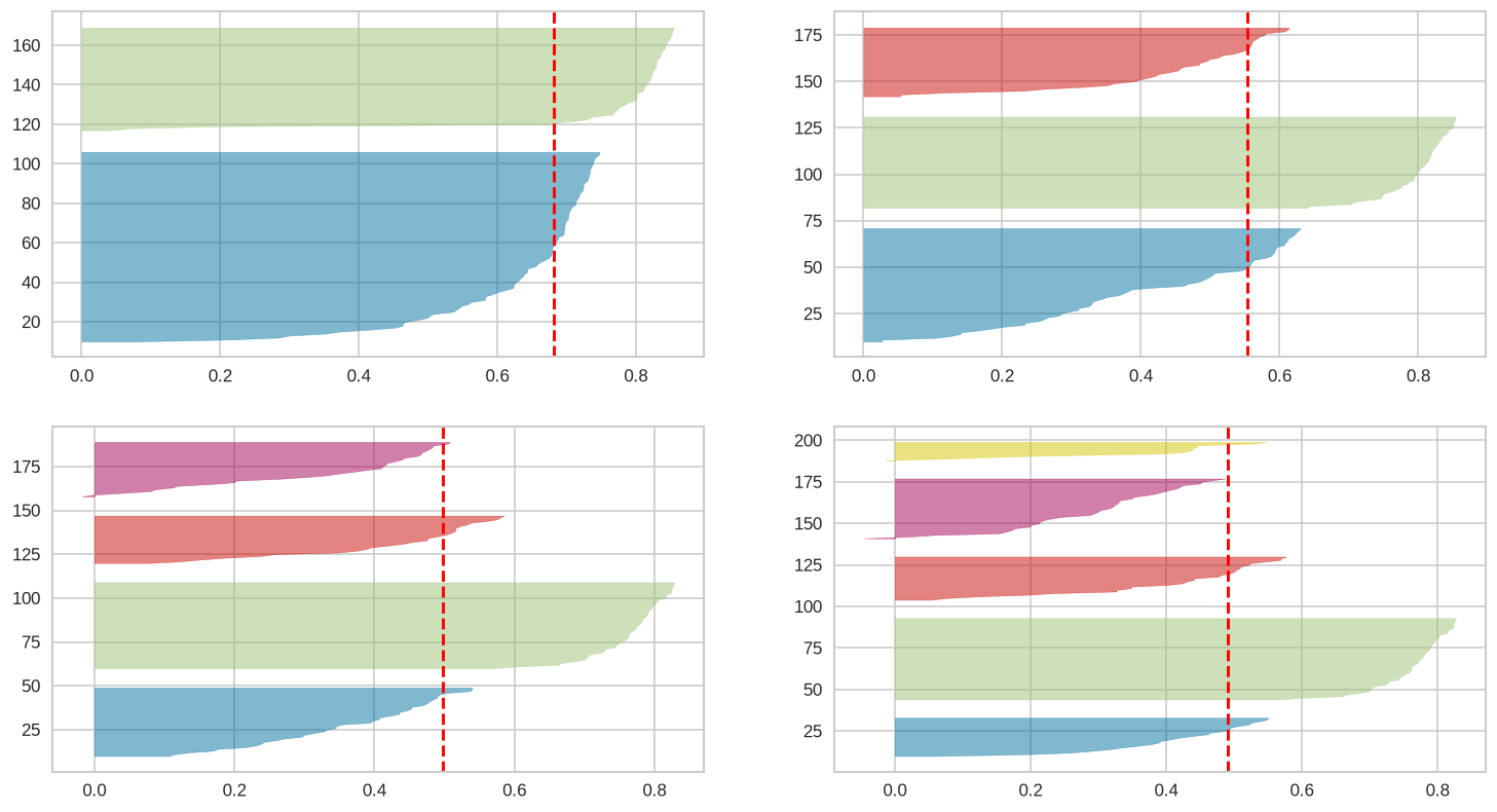
No single internal measure finds the true number of clusters. The silhouette sweep peaks at (about 0.68) while the ground truth has three classes (about 0.55). The silhouette rewards a coarse and well separated split, and “setosa versus the rest” is exactly that: a very clean two-group solution that is nevertheless not the classification. This is the key lesson of the session — an internal measure encodes a definition of a good cluster, not the truth. It can be optimised, and optimising it can select the wrong answer. Report several measures, look at the data, and trust a measure only when the question it encodes is the question you are asking.
The figure below is drawn with the yellowbrick package (pip install yellowbrick); the scores it prints are the same silhouette_score values computed above.
from yellowbrick.cluster import SilhouetteVisualizer
import matplotlib.pyplot as plt

fig, ax = plt.subplots(2, 2, figsize=(15,8))
scores = []
for i in [2, 3, 4, 5]:
    '''
    Create KMeans instance for different number of clusters
    '''
    km = KMeans(n_clusters=i, init='k-means++', n_init=10, max_iter=100, random_state=42)
    # Fit the KMeans model
    km.fit_predict(X)
    # Calculate Silhoutte Score
    score = silhouette_score(X, km.labels_, metric='euclidean')
    scores.append(score)
    q, mod = divmod(i, 2)
    '''
    Create SilhouetteVisualizer instance with KMeans instance
    Fit the visualizer
    '''
    visualizer = SilhouetteVisualizer(km, colors='yellowbrick', ax=ax[q-1][mod], force_model=True, is_fitted=True)
    visualizer.fit(X)

print({k: round(s, 3) for k, s in zip([2, 3, 4, 5], scores)})
{2: 0.681, 3: 0.553, 4: 0.498, 5: 0.491}
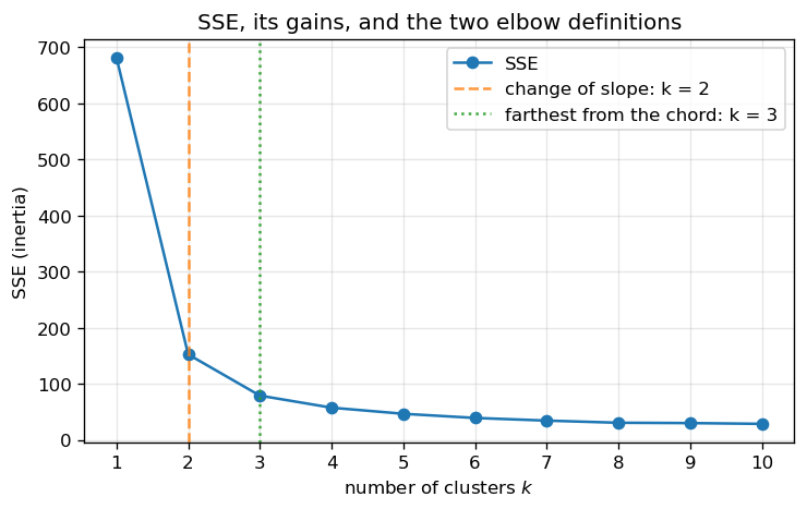
The SSE curve explains why the elbow rule is not a rule. The decrease is steep up to and then flattens, but it never stops decreasing: at large enough every point is its own cluster and the SSE is exactly zero.
ks = np.arange(1, 11)
sse = np.array([KMeans(n_clusters=int(k), random_state=42).fit(X).inertia_ for k in ks])

gains = -np.diff(sse)                 # SSE(k-1) - SSE(k)
slope = gains[:-1] - gains[1:]        # how much the gain itself shrinks

print(f"{'k':>2}  {'SSE':>8}  {'gain':>7}  {'slope change':>12}")
for k, value in zip(ks, sse):
    gain = f"{gains[k - 2]:7.2f}" if k > 1 else f"{'-':>7}"
    bend = f"{slope[k - 2]:12.2f}" if 2 <= k <= len(ks) - 1 else f"{'-':>12}"
    print(f"{k:>2}  {value:8.2f}  {gain}  {bend}")

knee_slope = int(ks[1 + np.argmax(slope)])
print(f"\nchange of slope          -> k = {knee_slope}  (drop {slope.max():.2f})")

# geometric variant (Kneedle): the point farthest from the chord joining the two ends
xn = (ks - ks.min()) / (ks.max() - ks.min())
yn = (sse - sse.min()) / (sse.max() - sse.min())
dy, dx = yn[-1] - yn[0], xn[-1] - xn[0]
distance = np.abs(dy * xn - dx * yn + xn[-1] * yn[0] - yn[-1] * xn[0]) / np.hypot(dy, dx)
knee_chord = int(ks[np.argmax(distance)])
print(f"farthest from the chord  -> k = {knee_chord}  "
      f"(distance {distance.max():.3f}, against {distance[1]:.3f} at k = 2)")

plt.figure(figsize=(7, 4))
plt.plot(ks, sse, marker="o", label="SSE")
plt.axvline(knee_slope, color="C1", ls="--", alpha=0.8,
            label=f"change of slope: k = {knee_slope}")
plt.axvline(knee_chord, color="C2", ls=":", alpha=0.9,
            label=f"farthest from the chord: k = {knee_chord}")
plt.xlabel("number of clusters $k$")
plt.ylabel("SSE (inertia)")
plt.title("SSE, its gains, and the two elbow definitions")
plt.xticks(ks)
plt.grid(alpha=0.3)
plt.legend()
plt.show()
 k       SSE     gain  slope change
 1    681.37        -             -
 2    152.35   529.02        455.53
 3     78.86    73.49         51.99
 4     57.35    21.50         10.63
 5     46.47    10.88          3.47
 6     39.07     7.41          2.65
 7     34.31     4.76          0.93
 8     30.48     3.83          3.26
 9     29.91     0.57         -0.79
10     28.55     1.36             -

change of slope          -> k = 2  (drop 455.53)
farthest from the chord  -> k = 3  (distance 0.495, against 0.494 at k = 2)
Choosing the Number of Clusters
None of the measures above returns by itself. The usual workflow is a sweep: cluster the data once for every candidate , compute a measure for each, and read the sequence. The silhouette and the gap statistic have a natural optimum — a peak, and a first crossing — while the SSE only decreases, so its curve needs a convention before it can be read. The oldest convention is the elbow.
The elbow rule
Run k-means for and plot the SSE against . Every new centroid can only lower the objective, so the curve falls monotonically; the question is where it stops falling fast. The intuition is that while the clusters are still being carved out of the data, each extra centroid removes a large part of the error, and afterwards it only splits groups that were already tight. The at the bend of the arm is the answer.
The bend is where the gain of one more centroid stops being worth it. Write the gain of going from to centroids as
While the curve is steep, each new centroid buys a lot; after the bend the next centroid buys much less than the previous one. The criterion is therefore the largest drop between two consecutive gains — the discrete second difference, or change of slope:
Dividing the same quantity by makes it unit-free and usually gives the same .
Do not use the largest relative gain as the criterion. Going from one centroid to two always removes by far the largest fraction of the error — the first centroid sits at the centre of the whole cloud — so that rule answers on almost every dataset, whatever the structure is.
The geometric version — Kneedle, from Satopää et al. (2011) — needs no threshold at all: it rescales both axes to , joins the first and the last point of the curve by a chord, and takes the point farthest from it.
where and are the rescaled coordinates. It depends on the range of the sweep, which the change-of-slope rule does not. Both versions are still heuristics: they turn a picture into a number, not into evidence.
With the change-of-slope rule the answer on Iris is : the gains are 529, 73, 21.5, 10.9, 7.4, 4.8, 3.8, 1 and 1, so the drop between consecutive gains falls from 455 to 52 to 11 and then to single digits — after the second centroid nothing comparable is left to win. The chord puts the bend one step further, at , but by 0.001 only (0.495 against 0.494 at ).
That near-tie is the honest lesson of the page, not a numerical accident: the curve describes the geometry of the data — one compact group (setosa) plus a spread-out remainder — and geometry does not contain a “true” number of classes. If the problem really has three species, that knowledge comes from the domain; the curve is at best consistent with it.
What the elbow rule is good for
It is cheap: one clustering per and no pairwise distances, so it scales to data where the silhouette does not.
It optimises exactly what k-means optimises. When compact, roughly spherical clusters are the goal, the bend is a defensible answer.
It cannot recover a that is not written into the geometry, it moves when the features are rescaled, and it should never be reported without the curve.
When the elbow is ambiguous, put it next to the silhouette sweep above (a peak, here at ) and to the gap statistic, which is worked out in the appendix together with NMI. If they still disagree, the data does not single out one : pick the one the downstream task can use.
Choosing the Right Metric
Use external measures when ground truth is available
Use internal measures when no labels exist
Consider multiple metrics together for robust evaluation
Remember that no single metric tells the whole story - different metrics may be more appropriate for different clustering goals.
Summary
A clustering needs validation: without labels, “it converged” says nothing about quality.
External measures start from the contingency table (row = cluster, column = class), computed in .
Purity is the sum of the row maxima; it is optimistic, because it allows two clusters to claim the same class.
Precision, recall and F add the column view; the maximum matching forces a one-to-one pairing and is an assignment problem (
linear_sum_assignment).Pairwise measures count agreements on pairs of points: Jaccard ignores , Rand counts everything and is inflated by , ARI corrects Rand for chance.
Internal measures — silhouette and SSE — use only the data; neither identifies the true number of clusters, and optimising one of them can give the wrong answer.
The elbow rule reads the SSE curve as a sequence of gains: the bend is where the next gain is much smaller than the current one. On Iris that is , the chord of the Kneedle variant says by a margin of 0.001, and the silhouette peaks at : a heuristic, not a verdict.
NMI, the gap statistic and the full assignment-problem treatment live in the appendix.
Report several measures, and state which question each of them answers.
- Zaki, M. J., & Meira, W. (2020). Data Mining and Machine Learning: Fundamental Concepts and Algorithms (2nd ed.). Cambridge University Press. https://www.cambridge.org/9781108497367