Model Selection

Model Selection
Can I trust you?
Mahmood Amintoosi, Fall 2026
Computer Science Dept, Ferdowsi University of Mashhad
I should mention that the original material of this course was from Open Machine Learning Course, by Joaquin Vanschoren and others.
Source
# Auto-setup when running on Google Colab
import os
if 'google.colab' in str(get_ipython()) and not os.path.exists('/content/machine-learning'):
    !git clone -q https://github.com/fum-cs/machine-learning.git /content/machine-learning
    !pip --quiet install -r /content/machine-learning/requirements_colab.txt
    %cd machine-learning/notebooks

# Global imports and settings
%matplotlib inline
from preamble import *
interactive = True # Set to True for interactive plots
if interactive:
    fig_scale = 0.9
    plt.rcParams.update(print_config)
else:
fig_scale = 1.25Evaluation
To know whether we can trust our method or system, we need to evaluate it.
Model selection: choose between different models in a data-driven way.
If you cannot measure it, you cannot improve it.
Convince others that your work is meaningful
Peers, leadership, clients, yourself(!)
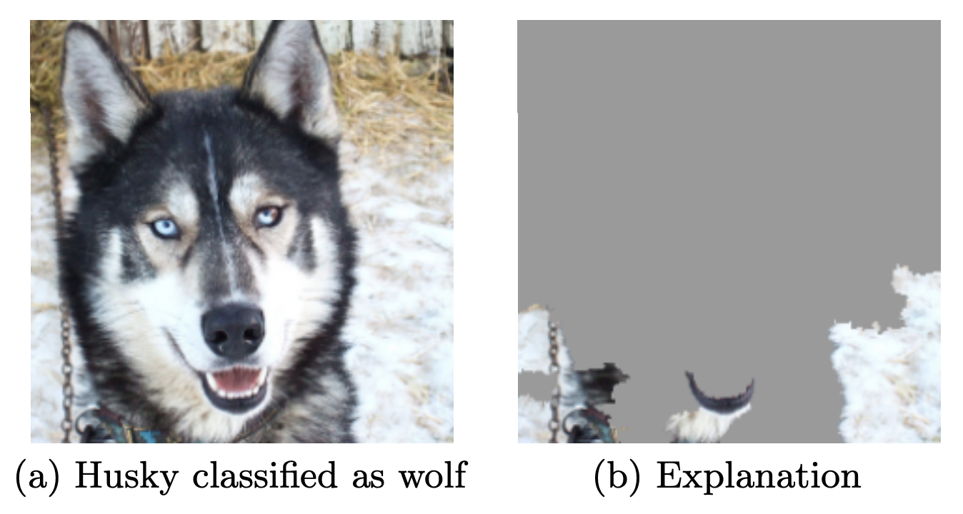
When possible, try to interpret what your model has learned
The signal your model found may just be an artifact of your biased data
See ‘Why Should I Trust You?’ by Marco Ribeiro et al.
Designing Machine Learning systems
Just running your favourite algorithm is usually not a great way to start
Consider the problem: How to measure success? Are there costs involved?
Do you want to understand phenomena or do black box modelling?
Analyze your model’s mistakes. Don’t just finetune endlessly.
Build early prototypes. Should you collect more, or additional data?
Should the task be reformulated?
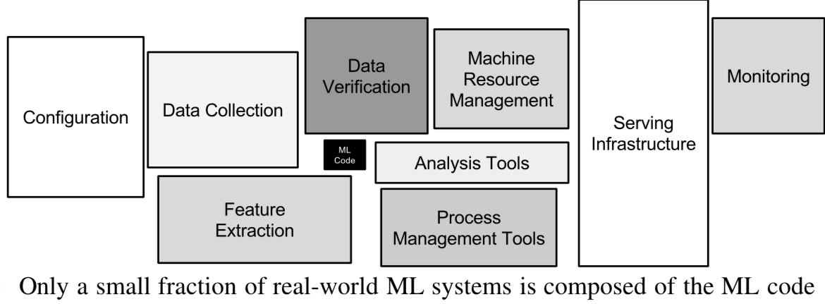
Overly complex machine learning systems are hard to maintain
See ‘Machine Learning: The High Interest Credit Card of Technical Debt’
Real world evaluations
Evaluate predictions, but also how outcomes improve because of them
Beware of feedback loops: predictions can influence future input data
Medical recommendations, spam filtering, trading algorithms,...
Evaluate algorithms in the wild.
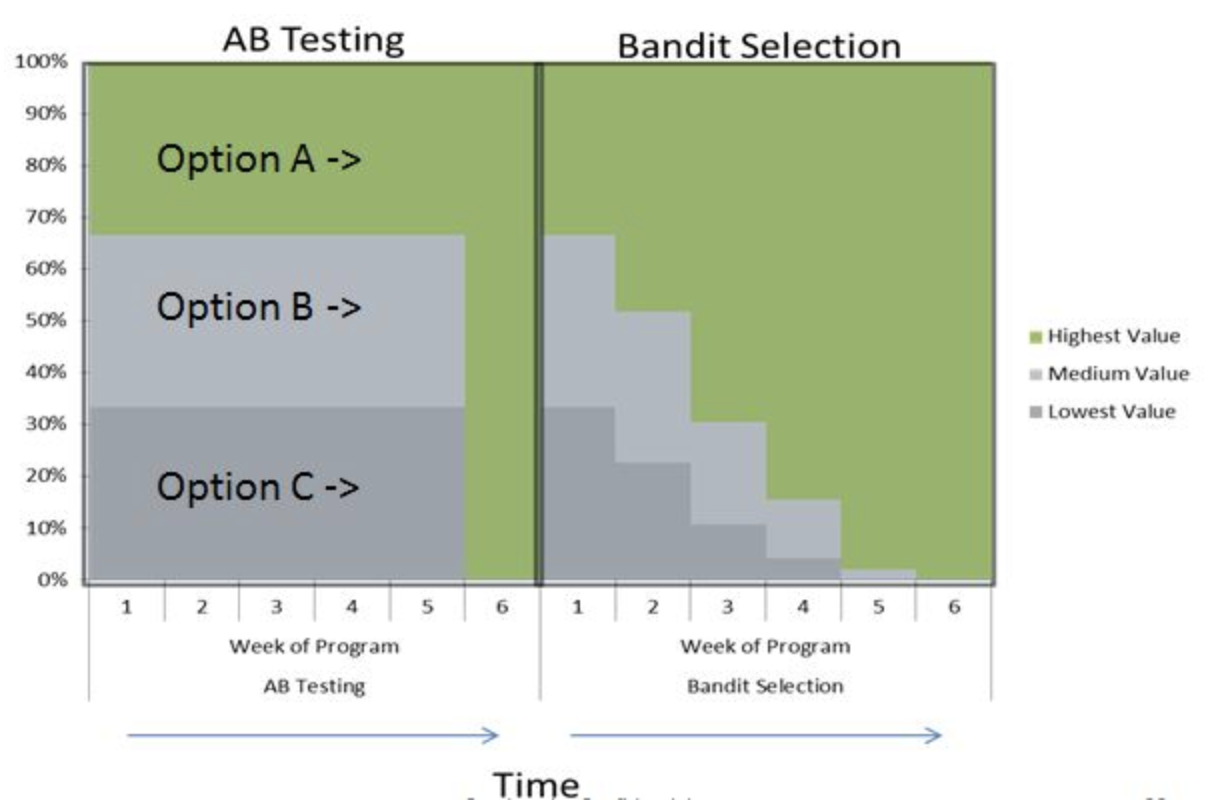
A/B testing: split users in groups, test different models in parallel
Bandit testing: gradually direct more users to the winning system
Performance estimation techniques
Always evaluate models as if they are predicting future data
We do not have access to future data, so we pretend that some data is hidden
Simplest way: the holdout (simple train-test split)
Randomly split data (and corresponding labels) into training and test set (e.g. 75%-25%)
Train (fit) a model on the training data, score on the test data
Source
from sklearn.model_selection import (TimeSeriesSplit, KFold, ShuffleSplit, train_test_split,
                                     StratifiedKFold, GroupShuffleSplit,
                                     GroupKFold, StratifiedShuffleSplit)
from matplotlib.patches import Patch
np.random.seed(1338)
cmap_data = plt.cm.brg
cmap_group = plt.cm.Paired
cmap_cv = plt.cm.coolwarm
n_splits = 4

# Generate the class/group data
n_points = 100
X = np.random.randn(100, 10)

percentiles_classes = [.1, .3, .6]
y = np.hstack([[ii] * int(100 * perc)
               for ii, perc in enumerate(percentiles_classes)])

# Evenly spaced groups repeated once
rng = np.random.RandomState(42)
group_prior = rng.dirichlet([2]*10)
rng.multinomial(100, group_prior)
groups = np.repeat(np.arange(10), rng.multinomial(100, group_prior))
Source
X_train, X_test, y_train, y_test = train_test_split(X, y, random_state=0)
fig, ax = plt.subplots(figsize=(8*fig_scale, 3*fig_scale))
mglearn.discrete_scatter(X_train[:, 0], X_train[:, 1], y_train,
                         markers='o', ax=ax)
mglearn.discrete_scatter(X_test[:, 0], X_test[:, 1], y_test,
                         markers='^', ax=ax)
ax.legend(["Train class 0", "Train class 1", "Train class 2", "Test class 0",
"Test class 1", "Test class 2"], ncol=6, loc=(-0.1, 1.1));K-fold Cross-validation
Each random split can yield very different models (and scores)
e.g. all easy (of hard) examples could end up in the test set
Split data into k equal-sized parts, called folds
Create k splits, each time using a different fold as the test set
Compute k evaluation scores, aggregate afterwards (e.g. take the mean)
Examine the score variance to see how sensitive (unstable) models are
Large k gives better estimates (more training data), but is expensive
Source
def plot_cv_indices(cv, X, y, group, ax, lw=2, show_groups=False, s=700, legend=True):
    """Create a sample plot for indices of a cross-validation object."""
    n_splits = cv.get_n_splits(X, y, group)

    # Generate the training/testing visualizations for each CV split
    for ii, (tr, tt) in enumerate(cv.split(X=X, y=y, groups=group)):
        # Fill in indices with the training/test groups
        indices = np.array([np.nan] * len(X))
        indices[tt] = 1
        indices[tr] = 0

        # Visualize the results
        ax.scatter([n_splits - ii - 1] * len(indices), range(len(indices)),
                   c=indices, marker='_', lw=lw, cmap=cmap_cv,
                   vmin=-.2, vmax=1.2, s=s)

    # Plot the data classes and groups at the end
    ax.scatter([-1] * len(X), range(len(X)),
               c=y, marker='_', lw=lw, cmap=cmap_data, s=s)
    yticklabels = ['class'] + list(range(1, n_splits + 1))

    if show_groups:
        ax.scatter([-2] * len(X), range(len(X)),
                   c=group, marker='_', lw=lw, cmap=cmap_group, s=s)
        yticklabels.insert(0, 'group')

    # Formatting
    ax.set(xticks=np.arange(-1 - show_groups, n_splits), xticklabels=yticklabels,
            ylabel='Sample index', xlabel="CV iteration",
            xlim=[-1.5 - show_groups, n_splits+.2], ylim=[-6, 100])
    ax.set_title('{}'.format(type(cv).__name__), fontsize=15)
    if legend:
        ax.legend([Patch(color=cmap_cv(.8)), Patch(color=cmap_cv(.2))],
                  ['Testing set', 'Training set'], loc=(1.02, .8))
    ax.spines['top'].set_visible(False)
    ax.spines['right'].set_visible(False)
    ax.spines['left'].set_visible(False)
    ax.spines['bottom'].set_visible(False)
    ax.set_yticks(())
    return ax
Source
fig, ax = plt.subplots(figsize=(6*fig_scale, 3*fig_scale))
cv = KFold(5)
plot_cv_indices(cv, X, y, groups, ax, s=700);Can you explain this result?
kfold = KFold(n_splits=3)
cross_val_score(logistic_regression, iris.data, iris.target, cv=kfold)
Source
from sklearn.model_selection import KFold, StratifiedKFold, cross_val_score
from sklearn.datasets import load_iris
from sklearn.linear_model import LogisticRegression

iris = load_iris()
logreg = LogisticRegression()
kfold = KFold(n_splits=3)
print("Cross-validation scores KFold(n_splits=3):\n{}".format(
      cross_val_score(logreg, iris.data, iris.target, cv=kfold)))
Cross-validation scores KFold(n_splits=3):
[0. 0. 0.]
Source
fig, ax = plt.subplots(figsize=(6*fig_scale, 3*fig_scale))
plot_cv_indices(kfold, iris.data, iris.target, iris.target, ax, s=700)
ax.set_ylim((-6, 150));Stratified K-Fold cross-validation
If the data is unbalanced, some classes have only few samples
Likely that some classes are not present in the test set
Stratification: proportions between classes are conserved in each fold
Order examples per class
Separate the samples of each class in k sets (strata)
Combine corresponding strata into folds
Source
fig, ax = plt.subplots(figsize=(6*fig_scale, 3*fig_scale))
cv = StratifiedKFold(5)
plot_cv_indices(cv, X, y, groups, ax, s=700)
ax.set_ylim((-6, 100));Leave-One-Out cross-validation
k fold cross-validation with k equal to the number of samples
Completely unbiased (in terms of data splits), but computationally expensive
Actually generalizes less well towards unseen data
The training sets are correlated (overlap heavily)
Overfits on the data used for (the entire) evaluation
A different sample of the data can yield different results
Recommended only for small datasets
Source
fig, ax = plt.subplots(figsize=(20*fig_scale, 4*fig_scale))
cv = KFold(33) # There are more than 33 classes, but this visualizes better.
plot_cv_indices(cv, X, y, groups, ax, s=700)
ax.set_ylim((-6, 100));Shuffle-Split cross-validation
Shuffles the data, samples (
train_size) points randomly as the training setCan also use a smaller (
test_size), handy with very large datasetsNever use if the data is ordered (e.g. time series)
Source
fig, ax = plt.subplots(figsize=(6*fig_scale, 3*fig_scale))
cv = ShuffleSplit(8, test_size=.2)
plot_cv_indices(cv, X, y, groups, ax, n_splits, s=700)
ax.set_ylim((-6, 100))
ax.legend([Patch(color=cmap_cv(.8)), Patch(color=cmap_cv(.2))],
['Testing set', 'Training set'], loc=(.95, .8));The Bootstrap
Sample n (dataset size) data points, with replacement, as training set (the bootstrap)
On average, bootstraps include 66% of all data points (some are duplicates)
Use the unsampled (out-of-bootstrap) samples as the test set
Repeat times to obtain scores
Similar to Shuffle-Split with
train_size=0.66,test_size=0.34but without duplicates
Source
from sklearn.utils import resample

# Toy implementation of bootstrapping
class Bootstrap:
    def __init__(self, nr):
        self.nr = nr

    def get_n_splits(self, X, y, groups=None):
        return self.nr

    def split(self, X, y, groups=None):
        indices = range(len(X))
        splits = []
        for i in range(self.nr):
            train = resample(indices, replace=True, n_samples=len(X), random_state=i)
            test = list(set(indices) - set(train))
            splits.append((train, test))
        return splits

fig, ax = plt.subplots(figsize=(6*fig_scale, 3*fig_scale))
cv = Bootstrap(8)
plot_cv_indices(cv, X, y, groups, ax, n_splits, s=700)
ax.set_ylim((-6, 100))
ax.legend([Patch(color=cmap_cv(.8)), Patch(color=cmap_cv(.2))],
['Testing set', 'Training set'], loc=(.95, .8));Repeated cross-validation
Cross-validation is still biased in that the initial split can be made in many ways
Repeated, or n-times-k-fold cross-validation:
Shuffle data randomly, do k-fold cross-validation
Repeat n times, yields n times k scores
Unbiased, very robust, but n times more expensive
Source
from sklearn.model_selection import RepeatedStratifiedKFold
from matplotlib.patches import Rectangle
fig, ax = plt.subplots(figsize=(10*fig_scale, 3*fig_scale))
cv = RepeatedStratifiedKFold(n_splits=5, n_repeats=3)
plot_cv_indices(cv, X, y, groups, ax, lw=2, s=400, legend=False)
ax.set_ylim((-6, 102))
xticklabels = ["class"] + [f"{repeat}x{split}" for repeat in range(1, 4) for split in range(1, 6)]
ax.set_xticklabels(xticklabels)
for i in range(3):
    rect = Rectangle((-.5 + i * 5, -2.), 5, 103, edgecolor='k', facecolor='none')
ax.add_artist(rect)Cross-validation with groups
Sometimes the data contains inherent groups:
Multiple samples from same patient, images from same person,...
Data from the same person may end up in the training and test set
We want to measure how well the model generalizes to other people
Make sure that data from one person are in either the train or test set
This is called grouping or blocking
Leave-one-subject-out cross-validation: test set for each subject/group
Source
fig, ax = plt.subplots(figsize=(6*fig_scale, 3*fig_scale))
cv = GroupKFold(5)
plot_cv_indices(cv, X, y, groups, ax, s=700, show_groups=True)
ax.set_ylim((-6, 100));Time series
When the data is ordered, random test sets are not a good idea
Source
import pandas as pd
approval = pd.read_csv("../data/approval_topline.csv")
adults = approval.groupby("subgroup").get_group('Adults')
adults = adults.set_index('modeldate')[::-1]
adults.approve_estimate.plot()
ax = plt.gca()
plt.rcParams["figure.figsize"] = (12*fig_scale,6*fig_scale)
ax.set_xlabel("")
xlim, ylim = ax.get_xlim(), ax.get_ylim()
for i in range(20):
    rect = Rectangle((np.random.randint(0, xlim[1]), ylim[0]), 10, ylim[1]-ylim[0], facecolor='#FFAAAA')
    ax.add_artist(rect)
plt.title("Presidential approval estimates by fivethirtyeight")
plt.legend([rect], ['Random Test Set'] );Test-then-train (prequential evaluation)
Every new sample is evaluated only once, then added to the training set
Can also be done in batches (of n samples at a time)
TimeSeriesSplitIn the kth split, the first k folds are the train set and the (k+1)th fold as the test set
Often, a maximum training set size (or window) is used
more robust against concept drift (change in data over time)
Source
from sklearn.utils import shuffle
fig, ax = plt.subplots(figsize=(6*fig_scale, 3*fig_scale))
cv = TimeSeriesSplit(5, max_train_size=20)
plot_cv_indices(cv, X, shuffle(y), groups, ax, s=700, lw=2)
ax.set_ylim((-6, 100))
ax.set_title("TimeSeriesSplit(5, max_train_size=20)");Choosing a performance estimation procedure
No strict rules, only guidelines:
Always use stratification for classification (sklearn does this by default)
Use holdout for very large datasets (e.g. >1.000.000 examples)
Or when learners don’t always converge (e.g. deep learning)
Choose k depending on dataset size and resources
Use leave-one-out for very small datasets (e.g. <100 examples)
Use cross-validation otherwise
Most popular (and theoretically sound): 10-fold CV
Literature suggests 5x2-fold CV is better
Use grouping or leave-one-subject-out for grouped data
Use train-then-test for time series
Evaluation Metrics for Classification
Evaluation vs Optimization
Each algorithm optimizes a given objective function (on the training data)
E.g. remember L2 loss in Ridge regression
The choice of function is limited by what can be efficiently optimized
However, we evaluate the resulting model with a score that makes sense in the real world
Percentage of correct predictions (on a test set)
The actual cost of mistakes (e.g. in money, time, lives,...)
We also tune the algorithm’s hyperparameters to maximize that score
Binary classification
We have a positive and a negative class
2 different kind of errors:
False Positive (type I error): model predicts positive while true label is negative
False Negative (type II error): model predicts negative while true label is positive
They are not always equally important
Which side do you want to err on for a medical test?

Confusion matrices
We can represent all predictions (correct and incorrect) in a confusion matrix
n by n array (n is the number of classes)
Rows correspond to true classes, columns to predicted classes
Count how often samples belonging to a class C are classified as C or any other class.
For binary classification, we label these true negative (TN), true positive (TP), false negative (FN), false positive (FP)
| Predicted Neg | Predicted Pos | |
|---|---|---|
| Actual Neg | TN | FP |
| Actual Pos | FN | TP |
Source
from sklearn.metrics import accuracy_score, confusion_matrix
from sklearn.model_selection import train_test_split
from sklearn.datasets import load_breast_cancer
from sklearn.linear_model import LogisticRegression
data = load_breast_cancer()
X_train, X_test, y_train, y_test = train_test_split(
    data.data, data.target, stratify=data.target, random_state=0)
lr = LogisticRegression().fit(X_train, y_train)
y_pred = lr.predict(X_test)

print("confusion_matrix(y_test, y_pred): \n", confusion_matrix(y_test, y_pred))
confusion_matrix(y_test, y_pred):
[[48 5]
[ 5 85]]
Predictive accuracy
Accuracy can be computed based on the confusion matrix
Not useful if the dataset is very imbalanced
E.g. credit card fraud: is 99.99% accuracy good enough?
3 models: very different predictions, same accuracy:
def plot_confusion_matrix(values, xlabel="predicted labels", ylabel="true labels", xticklabels=None,
                          yticklabels=None, cmap=None, vmin=None, vmax=None, ax=None,
                          fmt="{:.2f}", xtickrotation=45, norm=None, fsize=8):

    if ax is None:
        ax = plt.gca()
    ax.figure.set_size_inches(6*fig_scale, 6*fig_scale)
    values = np.array(values)  # Ensure 'values' is a numpy array for consistent handling
    img = ax.pcolormesh(values, cmap=cmap, vmin=vmin, vmax=vmax, norm=norm)
    ax.set_xlabel(xlabel, fontsize=8)
    ax.set_ylabel(ylabel, fontsize=8)

    # Setting the tick labels
    ax.set_xticks(np.arange(values.shape[1]) + 0.5, minor=False)
    ax.set_yticks(np.arange(values.shape[0]) + 0.5, minor=False)
    ax.set_xticklabels(xticklabels or [], minor=False, rotation=xtickrotation, fontsize=8)
    ax.set_yticklabels(yticklabels or [], minor=False, fontsize=8)

    # Loop over data dimensions and create text annotations.
    for i in range(values.shape[0]):
        for j in range(values.shape[1]):
            ax.text(j + 0.5, i + 0.5, fmt.format(values[i, j]),
                    ha="center", va="center", color="white" if values[i, j] > vmax/2 else "black", fontsize=8)

    ax.set_aspect('equal')  # Optional: set aspect ratio to be equal
    ax.invert_yaxis()
    return ax
Source
# Artificial 90-10 imbalanced target
y_true = np.zeros(100, dtype=int)
y_true[:10] = 1
y_pred_1 = np.zeros(100, dtype=int)
y_pred_2 = y_true.copy()
y_pred_2[10:20] = 1
y_pred_3 = y_true.copy()
y_pred_3[5:15] = 1 - y_pred_3[5:15]

def plot_measure(measure):
    fig, axes = plt.subplots(1, 3)
    for i, (ax, y_pred) in enumerate(zip(axes, [y_pred_1, y_pred_2, y_pred_3])):
        plot_confusion_matrix(confusion_matrix(y_true, y_pred), cmap='gray_r', ax=ax,
                              xticklabels=["N", "P"], yticklabels=["N", "P"], xtickrotation=0, vmin=0, vmax=100)
        ax.set_title("{}: {:.2f}".format(measure.__name__,measure(y_true, y_pred)), fontsize=8*fig_scale)

    plt.tight_layout()
Source
plot_measure(accuracy_score)Precision
Use when the goal is to limit FPs
Clinical trails: you only want to test drugs that really work
Search engines: you want to avoid bad search results
Source
from sklearn.metrics import precision_score
plot_measure(precision_score)Recall
Use when the goal is to limit FNs
Cancer diagnosis: you don’t want to miss a serious disease
Search engines: You don’t want to omit important hits
Also know as sensitivity, hit rate, true positive rate (TPR)
Source
from sklearn.metrics import recall_score
plot_measure(recall_score)Comparison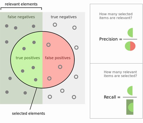
Source
from sklearn.metrics import f1_score
plot_measure(f1_score)Classification measure Zoo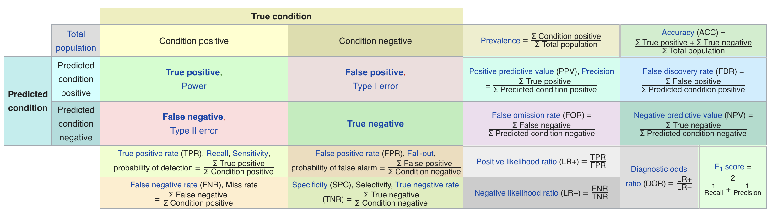
Multi-class classification
Train models per class : one class viewed as positive, other(s) als negative, then average
micro-averaging: count total TP, FP, TN, FN (every sample equally important)
micro-precision, micro-recall, micro-F1, accuracy are all the same
macro-averaging: average of scores obtained on each class
Preferable for imbalanced classes (if all classes are equally important)
macro-averaged recall is also called balanced accuracy
weighted averaging (: ratio of examples of class , aka support):
Source
from sklearn.metrics import classification_report

def report(y_pred):
    fig = plt.figure()
    ax = plt.subplot(111)
    plot_confusion_matrix(confusion_matrix(y_true, y_pred), cmap='gray_r', ax=ax,
                          xticklabels=["N", "P"], yticklabels=["N", "P"], xtickrotation=0, vmin=0, vmax=100, fsize=2.5)
    ax.figure.set_size_inches(2*fig_scale, 2*fig_scale)
    plt.gcf().text(1.1, 0.2, classification_report(y_true, y_pred), fontsize=8, fontname="Courier New")

    plt.tight_layout()
report(y_pred_1)
report(y_pred_2)
report(y_pred_3)Other useful classification metrics
Cohen’s Kappa
Measures ‘agreement’ between different models (aka inter-rater agreement)
To evaluate a single model, compare it against a model that does random guessing
Similar to accuracy, but taking into account the possibility of predicting the right class by chance
Can be weighted: different misclassifications given different weights
1: perfect prediction, 0: random prediction, negative: worse than random
With = accuracy, and = accuracy of random classifier:
Matthews correlation coefficient
Corrects for imbalanced data, alternative for balanced accuracy or AUROC
1: perfect prediction, 0: random prediction, -1: inverse prediction
Probabilistic evaluation
Classifiers can often provide uncertainty estimates of predictions.
Remember that linear models actually return a numeric value.
When , predict class -1, otherwise predict class +1
In practice, you are often interested in how certain a classifier is about each class prediction (e.g. cancer treatments).
Most learning methods can return at least one measure of confidence in their predicions.
Decision function: floating point value for each sample (higher: more confident)
Probability: estimated probability for each class
The decision function
In the binary classification case, the return value of the decision function encodes how strongly the model believes a data point belongs to the “positive” class.
Positive values indicate preference for the positive class.
The range can be arbitrary, and can be affected by hyperparameters. Hard to interpret.
Source
# create and split a synthetic dataset
from sklearn.linear_model import LogisticRegression
from sklearn.datasets import make_blobs
Xs, ys = make_blobs(centers=2, cluster_std=2.5, random_state=8)

# we rename the classes "blue" and "red"
ys_named = np.array(["blue", "red"])[ys]

# we can call train test split with arbitrary many arrays
# all will be split in a consistent manner
Xs_train, Xs_test, ys_train_named, ys_test_named, ys_train, ys_test = \
    train_test_split(Xs, ys_named, ys, random_state=0)

# build the logistic regression model
lr = LogisticRegression()
lr.fit(Xs_train, ys_train_named)

fig, axes = plt.subplots(1, 2, figsize=(10*fig_scale, 3.5*fig_scale))

mglearn.tools.plot_2d_separator(lr, Xs, ax=axes[0], alpha=.4,
                                fill=False, cm=mglearn.cm2)
scores_image = mglearn.tools.plot_2d_scores(lr, Xs, ax=axes[1],
                                            alpha=.4, cm=mglearn.ReBl)

for ax in axes:
    # plot training and test points
    mglearn.discrete_scatter(Xs_test[:, 0], Xs_test[:, 1], ys_test,
                             markers='^', ax=ax, s=7*fig_scale)
    mglearn.discrete_scatter(Xs_train[:, 0], Xs_train[:, 1], ys_train,
                             markers='o', ax=ax, s=7*fig_scale)
    ax.set_xlabel("Feature 0")
    ax.set_ylabel("Feature 1")
cbar = plt.colorbar(scores_image, ax=axes.tolist())
cbar.set_alpha(1)
cbar.ax.tick_params(labelsize=8*fig_scale)
axes[0].legend(["Test class 0", "Test class 1", "Train class 0",
"Train class 1"], ncol=4, loc=(.1, 1.1)); Predicting probabilities
Some models can also return a probability for each class with every prediction. These sum up to 1. We can visualize them again. Note that the gradient looks different now.
Source
fig, axes = plt.subplots(1, 2, figsize=(10*fig_scale, 3.5*fig_scale))

mglearn.tools.plot_2d_separator(
    lr, Xs, ax=axes[0], alpha=.4, fill=False, cm=mglearn.cm2)
scores_image = mglearn.tools.plot_2d_scores(
    lr, Xs, ax=axes[1], alpha=.5, cm=mglearn.ReBl, function='predict_proba')

for ax in axes:
    # plot training and test points
    mglearn.discrete_scatter(Xs_test[:, 0], Xs_test[:, 1], ys_test,
                             markers='^', ax=ax, s=7*fig_scale)
    mglearn.discrete_scatter(Xs_train[:, 0], Xs_train[:, 1], ys_train,
                             markers='o', ax=ax, s=7*fig_scale)
    ax.set_xlabel("Feature 0")
    ax.set_ylabel("Feature 1")
# don't want a transparent colorbar
cbar = plt.colorbar(scores_image, ax=axes.tolist())
cbar.set_alpha(1)
cbar.ax.tick_params(labelsize=8*fig_scale)
axes[0].legend(["Test class 0", "Test class 1", "Train class 0",
"Train class 1"], ncol=4, loc=(.1, 1.1));Threshold calibration
By default, we threshold at 0 for
decision_functionand 0.5 forpredict_probaDepending on the application, you may want to threshold differently
Lower threshold yields fewer FN (better recall), more FP (worse precision), and vice-versa
Source
from mglearn.datasets import make_blobs
from sklearn.svm import SVC
from sklearn.model_selection import train_test_split
from mglearn.tools import plot_2d_separator, plot_2d_scores, cm, discrete_scatter
import ipywidgets as widgets
from ipywidgets import interact, interact_manual

Xs, ys = make_blobs(n_samples=(400, 50), centers=2, cluster_std=[7.0, 2],
                    random_state=22)
Xs_train, Xs_test, ys_train, ys_test = train_test_split(Xs, ys, stratify=ys, random_state=0)
svc1 = SVC(gamma=.04).fit(Xs_train, ys_train)


@interact
def plot_decision_threshold(threshold=(-1.2,1.3,0.1)):
    fig, axes = plt.subplots(1, 2, figsize=(8*fig_scale, 2.2*fig_scale), subplot_kw={'xticks': (), 'yticks': ()})
    line = np.linspace(Xs_train.min(), Xs_train.max(), 100)

    axes[0].set_title("decision with threshold {:.2f}".format(threshold))
    discrete_scatter(Xs_train[:, 0], Xs_train[:, 1], ys_train, ax=axes[0], s=7*fig_scale)
    discrete_scatter(Xs_test[:, 0], Xs_test[:, 1], ys_test, ax=axes[0], markers='^', s=7*fig_scale)

    plot_2d_scores(svc1, Xs_train, function="decision_function", alpha=.7,
                   ax=axes[0], cm=mglearn.ReBl)
    plot_2d_separator(svc1, Xs_train, linewidth=3, ax=axes[0], threshold=threshold)
    axes[0].set_xlim(Xs_train[:, 0].min(), Xs_train[:, 0].max())
    axes[0].plot(line, np.array([10 for i in range(len(line))]), 'k:', linewidth=2)

    axes[1].set_title("cross-section with threshold {:.2f}".format(threshold))
    axes[1].plot(line, svc1.decision_function(np.c_[line, 10 * np.ones(100)]), c='k')
    dec = svc1.decision_function(np.c_[line, 10 * np.ones(100)])
    contour = (dec > threshold).reshape(1, -1).repeat(10, axis=0)
    axes[1].contourf(line, np.linspace(-1.5, 1.5, 10), contour, linewidth=2, alpha=0.4, cmap=cm)
    discrete_scatter(Xs_test[:, 0], Xs_test[:, 1]*0, ys_test, ax=axes[1], markers='^', s=7*fig_scale)

    axes[1].plot(line, np.array([threshold for i in range(len(line))]), 'r:', linewidth=3)
    axes[1].tick_params(labelsize=8*fig_scale)

    axes[0].set_xlim(Xs_train[:, 0].min(), Xs_train[:, 0].max())
    axes[1].set_xlim(Xs_train[:, 0].min(), Xs_train[:, 0].max())
    axes[1].set_ylim(-1.5, 1.5)
    axes[1].set_xticks(())
    axes[1].set_yticks(np.arange(-1.5, 1.5, 0.5))
    axes[1].yaxis.tick_right()
    axes[1].set_ylabel("Decision value")

    y_pred = svc1.decision_function(Xs_test)
    y_pred = y_pred > threshold
    axes[1].text(Xs_train.min()+1,1.2,"Precision: {:.4f}".format(precision_score(ys_test,y_pred)), size=7*fig_scale)
    axes[1].text(Xs_train.min()+1,0.9,"Recall: {:.4f}".format(recall_score(ys_test,y_pred)), size=7*fig_scale)
plt.tight_layout();Source
if not interactive:
    plot_decision_threshold(0)
    plot_decision_threshold(-0.9)
Precision-Recall curve
The best trade-off between precision and recall depends on your application
You can have arbitrary high recall, but you often want reasonable precision, too.
Plotting precision against recall for all possible thresholds yields a precision-recall curve
Change the treshold until you find a sweet spot in the precision-recall trade-off
Often jagged at high thresholds, when there are few positive examples left
Source
from sklearn.ensemble import RandomForestClassifier
from sklearn.metrics import precision_recall_curve

# create a similar dataset as before, but with more samples
# to get a smoother curve
Xp, yp = make_blobs(n_samples=(4000, 500), centers=2, cluster_std=[7.0, 2], random_state=22)
Xp_train, Xp_test, yp_train, yp_test = train_test_split(Xp, yp, random_state=0)
svc2 = SVC(gamma=.05).fit(Xp_train, yp_train)
rf2 = RandomForestClassifier(n_estimators=100).fit(Xp_train, yp_train)

@interact
def plot_PR_curve(threshold=(-3.19,1.4,0.1), model=[svc2, rf2]):
    if hasattr(model, "predict_proba"):
        precision, recall, thresholds = precision_recall_curve(
            yp_test, model.predict_proba(Xp_test)[:, 1])
    else:
        precision, recall, thresholds = precision_recall_curve(
            yp_test, model.decision_function(Xp_test))
    # find existing threshold closest to zero
    close_zero = np.argmin(np.abs(thresholds))
    plt.figure(figsize=(10*fig_scale,4*fig_scale))
    plt.plot(recall[close_zero], precision[close_zero], 'o', markersize=10,
             label="threshold zero", fillstyle="none", c='k', mew=2)
    plt.plot(recall, precision, lw=2, label="precision recall curve")

    if hasattr(model, "predict_proba"):
        yp_pred = model.predict_proba(Xp_test)[:, 1] > threshold
    else:
        yp_pred = model.decision_function(Xp_test) > threshold
    plt.plot(recall_score(yp_test,yp_pred), precision_score(yp_test,yp_pred), 'o', markersize=10, label="threshold {:.2f}".format(threshold))

    plt.ylabel("Precision")
    plt.xlabel("Recall")
plt.legend(loc="best", prop={"size":10});Source
if not interactive:
    plot_PR_curve(threshold=-0.99,model=svc2)
Model selection
Some models can achieve trade-offs that others can’t
Your application may require very high recall (or very high precision)
Choose the model that offers the best trade-off, given your application
The area under the PR curve (AUPRC) gives the best overall model
Source
from sklearn.metrics import auc
colors=['b','r','g','y']

def plot_PR_curves(models):

    plt.figure(figsize=(10*fig_scale,4*fig_scale))
    for i, model in enumerate(models):
        if hasattr(model, "predict_proba"):
            precision, recall, thresholds = precision_recall_curve(
                yp_test, model.predict_proba(Xp_test)[:, 1])
            close_zero = np.argmin(np.abs(thresholds-0.5))
        else:
            precision, recall, thresholds = precision_recall_curve(
                yp_test, model.decision_function(Xp_test))
            close_zero = np.argmin(np.abs(thresholds))

        plt.plot(recall, precision, lw=2, c=colors[i], label="PR curve {}, Area: {:.4f}".format(model, auc(recall, precision)))
        plt.plot(recall[close_zero], precision[close_zero], 'o', markersize=10,
                 fillstyle="none", c=colors[i], mew=2, label="Default threshold {}".format(model))
        plt.ylabel("Precision")
        plt.xlabel("Recall")
        plt.legend(loc="lower left", prop={"size":9});

#svc2 = SVC(gamma=0.01).fit(X_train, y_train)
plot_PR_curves([svc2, rf2])Hyperparameter effects
Of course, hyperparameters affect predictions and hence also the shape of the curve
Source
svc3 = SVC(gamma=0.01).fit(Xp_train, yp_train)
svc4 = SVC(gamma=1).fit(Xp_train, yp_train)
plot_PR_curves([svc3, svc2, svc4])Receiver Operating Characteristics (ROC)
Trade off true positive rate with false positive rate
Plotting TPR against FPR for all possible thresholds yields a Receiver Operating Characteristics curve
Change the treshold until you find a sweet spot in the TPR-FPR trade-off
Lower thresholds yield higher TPR (recall), higher FPR, and vice versa
Source
from sklearn.metrics import roc_curve

@interact
def plot_ROC_curve(threshold=(-3.19,1.4,0.1), model=[svc2, rf2]):
    if hasattr(model, "predict_proba"):
        fpr, tpr, thresholds = roc_curve(yp_test, model.predict_proba(Xp_test)[:, 1])
    else:
        fpr, tpr, thresholds = roc_curve(yp_test, model.decision_function(Xp_test))
    # find existing threshold closest to zero
    close_zero = np.argmin(np.abs(thresholds))
    plt.figure(figsize=(10*fig_scale,4*fig_scale))
    plt.plot(fpr[close_zero], tpr[close_zero], 'o', markersize=10, label="threshold zero", fillstyle="none", c='k', mew=2)
    plt.plot(fpr, tpr, lw=2, label="ROC curve")

    closest = np.argmin(np.abs(thresholds-threshold))
    plt.plot(fpr[closest], tpr[closest], 'o', markersize=10, label="threshold {:.2f}".format(threshold))

    plt.ylabel("TPR (recall)")
    plt.xlabel("FPR")
plt.legend(loc="best", prop={"size":10});Source
if not interactive:
plot_ROC_curve(threshold=-0.99,model=svc2)Visualization
Histograms show the amount of points with a certain decision value (for each class)
can be seen from the positive predictions (top histogram)
can be seen from the negative predictions (bottom histogram)
Source
# More data for a smoother curve
Xb, yb = make_blobs(n_samples=(4000, 4000), centers=2, cluster_std=[3, 3], random_state=7)
Xb_train, Xb_test, yb_train, yb_test = train_test_split(Xb, yb, random_state=0)
svc_roc = SVC(C=2).fit(Xb_train, yb_train)
probs_roc = svc_roc.decision_function(Xb_test)

@interact
def plot_roc_threshold(threshold=(-2,2,0.1)):
    fig = plt.figure(constrained_layout=True, figsize=(10*fig_scale,4*fig_scale))
    axes = []
    gs = fig.add_gridspec(2, 2)
    axes.append(fig.add_subplot(gs[0, :-1]))
    axes.append(fig.add_subplot(gs[1, :-1]))
    axes.append(fig.add_subplot(gs[:, 1]))

    n=50 # number of histogram bins
    color=['b','r']
    color_fill=['b','c','m','r']
    labels=['TN','FP','FN','TP']

    # Histograms
    for label in range(2):
        ps = probs_roc[yb_test == label] # get prediction for given label
        p, x = np.histogram(ps, bins=n) # bin it into n bins
        x = x[:-1] + (x[1] - x[0])/2 # convert bin edges to center
        axes[1-label].plot(x, p, c=color[label], lw=2)
        axes[1-label].fill_between(x[x<threshold], p[x<threshold], -5, facecolor=color_fill[2*label], label='{}: {}'.format(labels[2*label],np.sum(p[x<threshold])))
        axes[1-label].fill_between(x[x>=threshold], p[x>threshold], -5, facecolor=color_fill[2*label+1], label='{}: {}'.format(labels[2*label+1],np.sum(p[x>=threshold])))
        axes[1-label].set_title('Histogram of decision values for points with class {}'.format(label), fontsize=12*fig_scale)
        axes[1-label].legend(prop={"size":10})

    #ROC curve
    fpr, tpr, thresholds = roc_curve(yb_test, svc_roc.decision_function(Xb_test))
    axes[2].plot(fpr, tpr, lw=2, label="ROC curve", c='k')
    closest = np.argmin(np.abs(thresholds-threshold))
    axes[2].plot(fpr[closest], tpr[closest], 'o', markersize=10, label="threshold {:.2f}".format(threshold))

    axes[2].set_title('ROC curve', fontsize=12*fig_scale)
    axes[2].set_xlabel("FPR")
    axes[2].set_ylabel("TPR")
axes[2].legend(prop={"size":10})Source
if not interactive:
    plot_roc_threshold(threshold=-0.99)
Model selection
Again, some models can achieve trade-offs that others can’t
Your application may require minizing FPR (low FP), or maximizing TPR (low FN)
The area under the ROC curve (AUROC or AUC) gives the best overall model
Frequently used for evaluating models on imbalanced data
Random guessing (TPR=FPR) or predicting majority class (TPR=FPR=1): 0.5 AUC
Source
from sklearn.metrics import auc
from sklearn.dummy import DummyClassifier

def plot_ROC_curves(models):
    fig = plt.figure(figsize=(10*fig_scale,4*fig_scale))
    for i, model in enumerate(models):
        if hasattr(model, "predict_proba"):
            fpr, tpr, thresholds = roc_curve(
                yb_test, model.predict_proba(Xb_test)[:, 1])
            close_zero = np.argmin(np.abs(thresholds-0.5))
        else:
            fpr, tpr, thresholds = roc_curve(
                yb_test, model.decision_function(Xb_test))
            close_zero = np.argmin(np.abs(thresholds))
        plt.plot(fpr, tpr, lw=2, c=colors[i], label="ROC curve {}, Area: {:.4f}".format(model, auc(fpr, tpr)))
        plt.plot(fpr[close_zero], tpr[close_zero], 'o', markersize=10,
                 fillstyle="none", c=colors[i], mew=2) #label="Default threshold {}".format(model)
        plt.ylabel("TPR (recall)")
        plt.xlabel("FPR")
        plt.legend(loc="lower right",prop={"size":10});

svc = SVC(gamma=.1).fit(Xb_train, yb_train)
rf = RandomForestClassifier(n_estimators=100).fit(Xb_train, yb_train)
dc = DummyClassifier(strategy='most_frequent').fit(Xb_train, yb_train)
dc2 = DummyClassifier(strategy='uniform').fit(Xb_train, yb_train)
plot_ROC_curves([dc, dc2, svc, rf])Multi-class AUROC (or AUPRC)
We again need to choose between micro- or macro averaging TPR and FPR.
Micro-average if every sample is equally important (irrespective of class)
Macro-average if every class is equally important, especially for imbalanced data
Source
from itertools import cycle

from sklearn.metrics import roc_curve, auc
from sklearn.model_selection import train_test_split
from sklearn.preprocessing import label_binarize
from sklearn.multiclass import OneVsRestClassifier
from numpy import interp
from sklearn.metrics import roc_auc_score

# 3 class imbalanced data
Xi, yi = make_blobs(n_samples=(800, 500, 60), centers=3, cluster_std=[7.0, 2, 3.0], random_state=22)
sizes = [800, 500, 60]

# Binarize the output
yi = label_binarize(yi, classes=[0, 1, 2])
n_classes = yi.shape[1]
Xi_train, Xi_test, yi_train, yi_test = train_test_split(Xi, yi, test_size=.5, random_state=0)

# Learn to predict each class against the other
classifier = OneVsRestClassifier(SVC(probability=True))
y_score = classifier.fit(Xi_train, yi_train).decision_function(Xi_test)

# Compute ROC curve and ROC area for each class
fpr = dict()
tpr = dict()
roc_auc = dict()
for i in range(n_classes):
    fpr[i], tpr[i], _ = roc_curve(yi_test[:, i], y_score[:, i])
    roc_auc[i] = auc(fpr[i], tpr[i])

# Compute micro-average ROC curve and ROC area
fpr["micro"], tpr["micro"], _ = roc_curve(yi_test.ravel(), y_score.ravel())
roc_auc["micro"] = auc(fpr["micro"], tpr["micro"])

# First aggregate all false positive rates
all_fpr = np.unique(np.concatenate([fpr[i] for i in range(n_classes)]))

# Then interpolate all ROC curves at this points
mean_tpr = np.zeros_like(all_fpr)
for i in range(n_classes):
    mean_tpr += interp(all_fpr, fpr[i], tpr[i])

# Finally average it and compute AUC
mean_tpr /= n_classes

fpr["macro"] = all_fpr
tpr["macro"] = mean_tpr
roc_auc["macro"] = auc(fpr["macro"], tpr["macro"])

# Plot all ROC curves
plt.figure(figsize=(10*fig_scale,4*fig_scale))

plt.plot(fpr["micro"], tpr["micro"],
         label='micro-average ROC curve (area = {0:0.2f})'
               ''.format(roc_auc["micro"]),
         color='deeppink', linestyle=':', linewidth=4)

plt.plot(fpr["macro"], tpr["macro"],
         label='macro-average ROC curve (area = {0:0.2f})'
               ''.format(roc_auc["macro"]),
         color='navy', linestyle=':', linewidth=4)

colors = cycle(['aqua', 'darkorange', 'cornflowerblue'])
for i, color in zip(range(n_classes), colors):
    plt.plot(fpr[i], tpr[i], color=color, lw=2, linestyle='-',
             label='ROC curve of class {} (size: {}) (area = {:0.2f})'
             ''.format(i, sizes[i], roc_auc[i]))

plt.plot([0, 1], [0, 1], 'k--', lw=2)
plt.xlim([0.0, 1.0])
plt.ylim([0.0, 1.05])
plt.xlabel('False Positive Rate')
plt.ylabel('True Positive Rate')
plt.title('Extension of ROC to multi-class')
plt.legend(loc="lower right", prop={"size":10})
plt.show()Model calibration
For some models, the predicted uncertainty does not reflect the actual uncertainty
If a model is 90% sure that samples are positive, is it also 90% accurate on these?
A model is called calibrated if the reported uncertainty actually matches how correct it is
Overfitted models also tend to be over-confident
LogisticRegression models are well calibrated since they learn probabilities
SVMs are not well calibrated. Biased towards points close to the decision boundary.
Source
from sklearn.svm import SVC
from sklearn.datasets import make_classification
from sklearn.calibration import calibration_curve
from sklearn.metrics import brier_score_loss, accuracy_score

def load_data():
    X, y = make_classification(n_samples=100000, n_features=20, random_state=0)
    train_samples = 2000  # Samples used for training the models
    X_train = X[:train_samples]
    X_test = X[train_samples:]
    y_train = y[:train_samples]
    y_test = y[train_samples:]

    return X_train, X_test, y_train, y_test

Xc_train, Xc_test, yc_train, yc_test = load_data()

def plot_calibration_curve(y_true, y_prob, n_bins=5, ax=None, hist=True, normalize=False):
    prob_true, prob_pred = calibration_curve(y_true, y_prob, n_bins=n_bins)
    if ax is None:
        ax = plt.gca()
    if hist:
        ax.hist(y_prob, weights=np.ones_like(y_prob) / len(y_prob), alpha=.4,
               bins=np.maximum(10, n_bins))
    ax.plot([0, 1], [0, 1], ':', c='k')
    curve = ax.plot(prob_pred, prob_true, marker="o")

    ax.set_xlabel("predicted probability")
    ax.set_ylabel("fraction of pos. samples")
    ax.set(aspect='equal')
    return curve

# Plot calibration curves for `models`, optionally show a calibrator run on a calibratee
def plot_calibration_comparison(models, calibrator=None, calibratee=None):
    def get_probabilities(clf, X):
        if hasattr(clf, "predict_proba"): # Use probabilities if classifier has predict_proba
            prob_pos = clf.predict_proba(X)[:, 1]
        else:  # Otherwise, use decision function and scale
            prob_pos = clf.decision_function(X)
            prob_pos = (prob_pos - prob_pos.min()) / (prob_pos.max() - prob_pos.min())
        return prob_pos

    nr_plots = len(models)
    if calibrator:
        nr_plots += 1
    fig, axes = plt.subplots(1, nr_plots, figsize=(3*nr_plots*fig_scale, 4*nr_plots*fig_scale))
    for ax, clf in zip(axes[:len(models)], models):
            clf.fit(Xc_train, yc_train)
            prob_pos = get_probabilities(clf,Xc_test)
            bs = brier_score_loss(yc_test,prob_pos)
            plot_calibration_curve(yc_test, prob_pos, n_bins=20, ax=ax)
            ax.set_title(clf.__class__.__name__, fontsize=10*fig_scale)
            ax.text(0,0.95,"Brier score: {:.3f}".format(bs), size=10*fig_scale)
    if calibrator:
        calibratee.fit(Xc_train, yc_train)
        # We're visualizing the trained calibrator, hence let it predict the training data
        prob_pos = get_probabilities(calibratee, Xc_train) # get uncalibrated predictions
        y_sort = [x for _,x in sorted(zip(prob_pos,yc_train))] # sort for nicer plots
        prob_pos.sort()
        cal_prob = calibrator.fit(prob_pos, y_sort).predict(prob_pos) # fit calibrator
        axes[-1].scatter(prob_pos,y_sort, s=2)
        axes[-1].scatter(prob_pos,cal_prob, s=2)
        axes[-1].plot(prob_pos,cal_prob)
        axes[-1].set_title("Calibrator: {}".format(calibrator.__class__.__name__), fontsize=10*fig_scale)
        axes[-1].set_xlabel("predicted probability")
        axes[-1].set_ylabel("outcome")
        axes[-1].set(aspect='equal')
    plt.tight_layout()

plot_calibration_comparison([LogisticRegression(), SVC()]) Brier score
You may want to select models based on how accurate the class confidences are.
The Brier score loss: squared loss between predicted probability and actual outcome
Lower is better
Source
from sklearn.datasets import load_breast_cancer
cancer = load_breast_cancer()
XC_train, XC_test, yC_train, yC_test = train_test_split(cancer.data, cancer.target, test_size=.5, random_state=0)

# LogReg
logreg = LogisticRegression().fit(XC_train, yC_train)
probs = logreg.predict_proba(XC_test)[:,1]
print("Logistic Regression Brier score loss: {:.4f}".format(brier_score_loss(yC_test,probs)))

# SVM: scale decision functions
svc = SVC().fit(XC_train, yC_train)
prob_pos = svc.decision_function(XC_test)
prob_pos = (prob_pos - prob_pos.min()) / (prob_pos.max() - prob_pos.min())
print("SVM Brier score loss: {:.4f}".format(brier_score_loss(yC_test,prob_pos)))
Logistic Regression Brier score loss: 0.0322
SVM Brier score loss: 0.0795
Model calibration techniques
We can post-process trained models to make them more calibrated.
Fit a regression model (a calibrator) to map the model’s outcomes to a calibrated probability in [0,1]
returns the decision values or probability estimates
is fitted on the training data to map these to the correct outcome
Often an internal cross-validation with few folds is used
Multi-class models require one calibrator per class
Source
from sklearn.calibration import CalibratedClassifierCV
from sklearn.linear_model import LogisticRegression

# Wrapped LogisticRegression to get sigmoid predictions
class Sigmoid():
    model = LogisticRegression()

    def fit(self, X, y):
        self.model.fit(X.reshape(-1, 1),y)
        return self

    def predict(self, X):
        return self.model.predict_proba(X.reshape(-1, 1))[:, 1]

svm = SVC()
svm_platt = CalibratedClassifierCV(svm, cv=2, method='sigmoid')
plot_calibration_comparison([svm, svm_platt],Sigmoid(),svm)Isotonic regression
Maps input to an output so that increases monotonically with and minimizes loss
Predictions are made by interpolating the predicted
Fit to minimize the loss between the uncalibrated predictions and the actual labels
Corrects any monotonic distortion, but tends to overfit on small samples
Source
from sklearn.isotonic import IsotonicRegression

model = SVC()
iso = CalibratedClassifierCV(model, cv=2, method='isotonic')
plot_calibration_comparison([model, iso],IsotonicRegression(),model)Cost-sensitive classification (dealing with imbalance)
In the real world, different kinds of misclassification can have different costs
Misclassifying certain classes can be more costly than others
Misclassifying certain samples can be more costly than others
Cost-sensitive resampling: resample (or reweight) the data to represent real-world expectations
oversample minority classes (or undersample majority) to ‘correct’ imbalance
increase weight of misclassified samples (e.g. in boosting)
decrease weight of misclassified (noisy) samples (e.g. in model compression)
Class weighting
If some classes are more important than others, we can give them more weight
E.g. for imbalanced data, we can give more weight to minority classes
Most classification models can include it in their loss function and optimize for it
E.g. Logistic regression: add a class weight in the log loss function
Source
def plot_decision_function(classifier, X, y, sample_weight, axis, title):
    # plot the decision function
    xx, yy = np.meshgrid(np.linspace(np.min(X[:,0])-1, np.max(X[:,0])+1, 500), np.linspace(np.min(X[:,1])-1, np.max(X[:,1])+1, 500))
    Z = classifier.decision_function(np.c_[xx.ravel(), yy.ravel()])
    Z = Z.reshape(xx.shape)

    # plot the line, the points, and the nearest vectors to the plane
    axis.contourf(xx, yy, Z, alpha=0.75, cmap=plt.cm.bone)
    axis.scatter(X[:, 0], X[:, 1], c=y, s=100 * sample_weight, alpha=0.9,
                 cmap=plt.cm.bone, edgecolors='black')

    axis.axis('off')
    axis.set_title(title)

def plot_class_weights():
    X, y = make_blobs(n_samples=(50, 10), centers=2, cluster_std=[7.0, 2], random_state=4)

    # fit the models
    clf_weights = SVC(gamma=0.1, C=0.1, class_weight={1: 10}).fit(X, y)
    clf_no_weights = SVC(gamma=0.1, C=0.1).fit(X, y)

    fig, axes = plt.subplots(1, 2, figsize=(9*fig_scale, 4*fig_scale))
    plot_decision_function(clf_no_weights, X, y, 1, axes[0],
                           "Constant weights")
    plot_decision_function(clf_weights, X, y, 1, axes[1],
                           "Modified class weights")
plot_class_weights()Instance weighting
If some training instances are important to get right, we can give them more weight
E.g. when some examples are from groups underrepresented in the data
These are passed during training (fit), and included in the loss function
E.g. Logistic regression: add a instance weight in the log loss function
Source
# Example from https://scikit-learn.org/stable/auto_examples/svm/plot_weighted_samples.html
def plot_instance_weights():
    np.random.seed(0)
    X = np.r_[np.random.randn(10, 2) + [1, 1], np.random.randn(10, 2)]
    y = [1] * 10 + [-1] * 10
    sample_weight_last_ten = abs(np.random.randn(len(X)))
    sample_weight_constant = np.ones(len(X))
    # and bigger weights to some outliers
    sample_weight_last_ten[15:] *= 5
    sample_weight_last_ten[9] *= 15

    # for reference, first fit without sample weights

    # fit the model
    clf_weights = SVC(gamma=1)
    clf_weights.fit(X, y, sample_weight=sample_weight_last_ten)

    clf_no_weights = SVC(gamma=1)
    clf_no_weights.fit(X, y)

    fig, axes = plt.subplots(1, 2, figsize=(9*fig_scale, 4*fig_scale))
    plot_decision_function(clf_no_weights, X, y, sample_weight_constant, axes[0],
                           "Constant weights")
    plot_decision_function(clf_weights, X, y, sample_weight_last_ten, axes[1],
                           "Modified instance weights")
plot_instance_weights() Cost-sensitive algorithms
Cost-sensitive algorithms
If misclassification cost of some classes is higher, we can give them higher weights
Some support cost matrix : costs for every possible type of error
Cost-sensitive ensembles: convert cost-insensitive classifiers into cost-sensitive ones
MetaCost: Build a model (ensemble) to learn the class probabilities
Relabel training data to minimize expected cost:
Accuracy may decrease but cost decreases as well.
AdaCost: Boosting with reweighting instances to reduce costs
Tuning the decision threshold
If every FP or FN has a certain cost, we can compute the total cost for a given model:
This yields different isometrics (lines of equal cost) in ROC space
Optimal threshold is the point on the ROC curve where cost is minimal (line search)
Source
import ipywidgets as widgets
from ipywidgets import interact, interact_manual

# Cost function
def cost(fpr, tpr, cost_FN, cost_FP, ratio_P):
    return fpr * cost_FP * ratio_P + (1 - tpr) * (1-ratio_P) * cost_FN;

@interact
def plot_isometrics(cost_FN=(1,10.0,1.0), cost_FP=(1,10.0,1.0)):
    from sklearn.metrics import roc_curve
    fpr, tpr, thresholds = roc_curve(yb_test, svc_roc.decision_function(Xb_test))

    # get minimum
    ratio_P = len(yb_test[yb_test==1]) / len(yb_test)
    costs = [cost(fpr[x],tpr[x],cost_FN,cost_FP, ratio_P) for x in range(len(thresholds))]
    min_cost = np.min(costs)
    min_thres = np.argmin(costs)

    # plot contours
    x = np.arange(0.0, 1.1, 0.1)
    y = np.arange(0.0, 1.1, 0.1)
    XX, YY = np.meshgrid(x, y)
    costs = [cost(f, t, cost_FN, cost_FP, ratio_P) for f, t in zip(XX,YY)]

    if interactive:
        fig, axes = plt.subplots(1, 1, figsize=(9*fig_scale, 3*fig_scale))
    else:
        fig, axes = plt.subplots(1, 1, figsize=(6*fig_scale, 1.8*fig_scale))
    plt.plot(fpr, tpr, label="ROC Curve", lw=2)
    levels = np.linspace(np.array(costs).min(), np.array(costs).max(), 10)
    levels = np.sort(np.append(levels, min_cost))
    CS = plt.contour(XX, YY, costs, levels)
    plt.clabel(CS, inline=1, fontsize=10)

    plt.xlabel("FPR")
    plt.ylabel("TPR (recall)")
    # find threshold closest to zero:
    plt.plot(fpr[min_thres], tpr[min_thres], 'o', markersize=4,
             label="optimal", fillstyle="none", c='k', mew=2)
    plt.legend(loc=4, prop={"size":10});
    plt.title("Isometrics, cost_FN: {}, cost_FP: {}".format(cost_FN, cost_FP), fontsize=10*fig_scale)
    plt.tight_layout()
plt.show()Source
if not interactive:
    plot_isometrics(1,1)
    plot_isometrics(1,9)
Regression metrics
Most commonly used are
mean squared error:
root mean squared error (RMSE) often used as well
mean absolute error:
Less sensitive to outliers and large errors
R squared
Ratio of variation explained by the model / total variation
Between 0 and 1, but negative if the model is worse than just predicting the mean
Easier to interpret (higher is better).
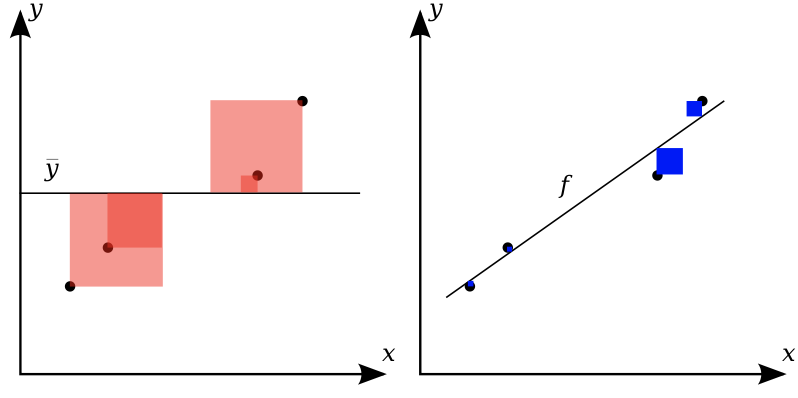
Visualizing regression errors
Prediction plot (left): predicted vs actual target values
Residual plot (right): residuals vs actual target values
Over- and underpredictions can be given different costs
Source
from sklearn.linear_model import Ridge
from sklearn.datasets import fetch_openml
from sklearn.pipeline import make_pipeline
from sklearn.preprocessing import StandardScaler
boston = fetch_openml(name="boston", as_frame=True)

X_train, X_test, y_train, y_test = train_test_split(boston.data, boston.target)
ridge_pipe = make_pipeline(StandardScaler(),Ridge())

pred = ridge_pipe.fit(X_train, y_train).predict(X_test)

plt.subplot(1, 2, 1)
plt.gca().set_aspect("equal")
plt.plot([10, 50], [10, 50], '--', c='k')
plt.plot(y_test, pred, 'o', alpha=.5, markersize=7*fig_scale)
plt.ylabel("predicted", fontsize=10*fig_scale)
plt.xlabel("true", fontsize=10*fig_scale);

plt.subplot(1, 2, 2)
plt.gca().set_aspect("equal")
plt.plot([10, 50], [0,0], '--', c='k')
plt.plot(y_test, y_test - pred, 'o', alpha=.5, markersize=7*fig_scale)
plt.xlabel("true", fontsize=10*fig_scale)
plt.ylabel("true - predicted", fontsize=10*fig_scale)
plt.tight_layout();Bias-Variance decomposition
Evaluate the same algorithm multiple times on different random samples of the data
Two types of errors can be observed:
Bias error: systematic error, independent of the training sample
These points are predicted (equally) wrong every time
Variance error: error due to variability of the model w.r.t. the training sample
These points are sometimes predicted accurately, sometimes inaccurately
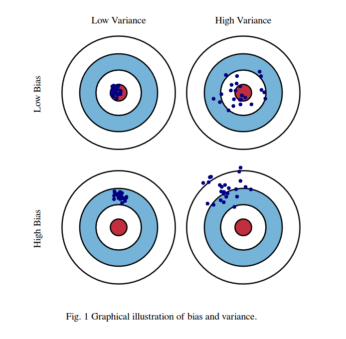
Computing bias and variance error
Take 100 or more bootstraps (or shuffle-splits)
Regression: for each data point x:
Classification: for each data point x:
= misclassification ratio
is ratio of class predictions
Total bias: : the percentage of times occurs in the test sets
Total variance:
Source
from sklearn.model_selection import ShuffleSplit, train_test_split, GridSearchCV

# Bias-Variance Computation
def compute_bias_variance(clf, X, y):
    # Bootstraps
    n_repeat = 40 # 40 is on the low side to get a good estimate. 100 is better.
    shuffle_split = ShuffleSplit(test_size=0.33, n_splits=n_repeat, random_state=0)

    # Store sample predictions
    y_all_pred = [[] for _ in range(len(y))]

    # Train classifier on each bootstrap and score predictions
    for i, (train_index, test_index) in enumerate(shuffle_split.split(X)):
        # Train and predict
        clf.fit(X[train_index], y[train_index])
        y_pred = clf.predict(X[test_index])

        # Store predictions
        for j,index in enumerate(test_index):
            y_all_pred[index].append(y_pred[j])

    # Compute bias, variance, error
    bias_sq = sum([ (1 - x.count(y[i])/len(x))**2 * len(x)/n_repeat
                for i,x in enumerate(y_all_pred)])
    var = sum([((1 - ((x.count(0)/len(x))**2 + (x.count(1)/len(x))**2))/2) * len(x)/n_repeat
               for i,x in enumerate(y_all_pred)])
    error = sum([ (1 - x.count(y[i])/len(x)) * len(x)/n_repeat
            for i,x in enumerate(y_all_pred)])

    return np.sqrt(bias_sq), var, error
Bias and variance, underfitting and overfitting
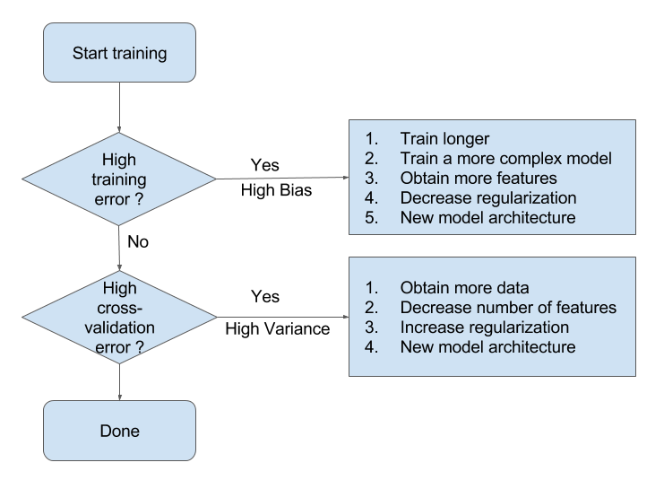
High variance means that you are likely overfitting
Use more regularization or use a simpler model
High bias means that you are likely underfitting
Do less regularization or use a more flexible/complex model
Ensembling techniques (see later) reduce bias or variance directly
Bagging (e.g. RandomForests) reduces variance, Boosting reduces bias
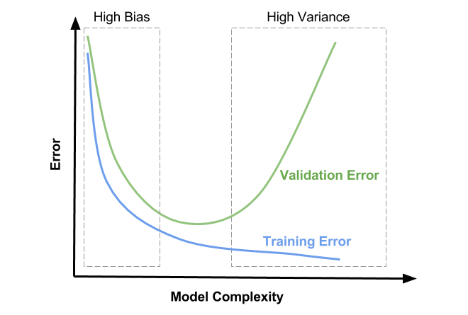
Understanding under- and overfitting
Regularization reduces variance error (increases stability of predictions)
But too much increases bias error (inability to learn ‘harder’ points)
High regularization (left side): Underfitting, high bias error, low variance error
High training error and high test error
Low regularization (right side): Overfitting, low bias error, high variance error
Low training error and higher test error
Source
from sklearn.datasets import load_breast_cancer
from sklearn.ensemble import RandomForestClassifier, AdaBoostClassifier
cancer = load_breast_cancer()

def plot_bias_variance(clf, param, X, y, ax):
    bias_scores = []
    var_scores = []
    err_scores = []
    name, vals = next(iter(param.items()))

    for i in vals:
        b,v,e = compute_bias_variance(clf.set_params(**{name:i}),X,y)
        bias_scores.append(b)
        var_scores.append(v)
        err_scores.append(e)

    ax.set_title(clf.__class__.__name__)
    ax.plot(vals, var_scores,label ="variance", lw=2 )
    ax.plot(vals, bias_scores,label ="bias", lw=2 )
    ax.set_xscale('log')
    ax.set_xlabel(name)
    ax.legend(loc="best")

def plot_train_test(clf, param, X, y, ax):
    gs = GridSearchCV(clf, param, cv=5, return_train_score=True).fit(X,y)
    name, vals = next(iter(param.items()))

    ax.set_title(clf.__class__.__name__)
    ax.plot(vals, (1-gs.cv_results_['mean_train_score']),label ="train error", lw=2 )
    ax.plot(vals, (1-gs.cv_results_['mean_test_score']),label ="test error", lw=2 )
    ax.set_xscale('log')
    ax.set_xlabel(name)
    ax.legend(loc="best")

fig, axes = plt.subplots(2, 2, figsize=(6*fig_scale, 4*fig_scale))
X, y = cancer.data, cancer.target
svm = SVC(gamma=2e-4, random_state=0)
param = {'C': [1e-4, 1e-2, 1, 1e2, 1e4]}

plot_bias_variance(svm, param, X, y, axes[0,1])
plot_train_test(svm, param, X, y, axes[1,1])

lr = LogisticRegression(random_state=0)
param = {'C': [1e-2, 1, 92, 1e4, 1e6]}
plot_bias_variance(lr, param, X, y, axes[0,0])
plot_train_test(lr, param, X, y, axes[1,0])
plt.tight_layout()Summary Flowchart (by Andrew Ng)
Hyperparameter tuning
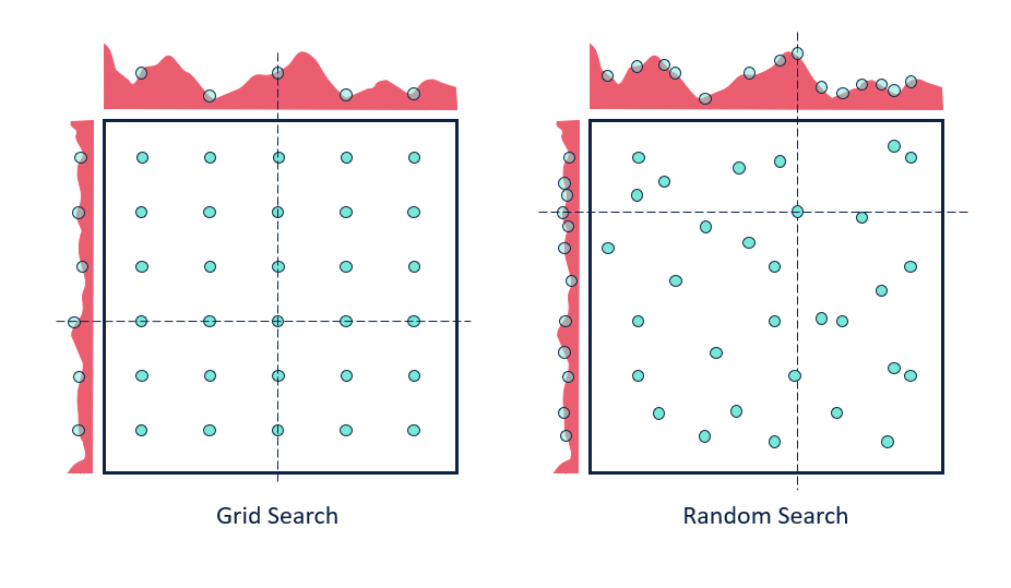
There exists a huge range of techniques to tune hyperparameters. The simplest:
Grid search: Choose a range of values for every hyperparameter, try every combination
Doesn’t scale to many hyperparameters (combinatorial explosion)
Random search: Choose random values for all hyperparameters, iterate times
Better, especially when some hyperparameters are less important
Many more advanced techniques exist, see lecture on Automated Machine Learning
First, split the data in training and test sets (outer split)
Split up the training data again (inner cross-validation)
Generate hyperparameter configurations (e.g. random/grid search)
Evaluate all configurations on all inner splits, select the best one (on average)
Retrain best configurations on full training set, evaluate on held-out test data
Source
if interactive:
    plt.rcParams['figure.dpi'] = 75
mglearn.plots.plot_grid_search_overview()
plt.rcParams.update(print_config)Source
from scipy.stats.distributions import exponNested cross-validation
Simplest approach: single outer split and single inner split (shown below)
Risk of over-tuning hyperparameters on specific train-test split
Only recommended for very large datasets
Nested cross-validation:
Outer loop: split full dataset in training and test splits
Inner loop: split training data into train and validation sets
This yields scores for possibly different hyperparameter settings
Average score is the expected performance of the tuned model
To use the model in practice, retune on the entire dataset
hps = {'C': expon(scale=100), 'gamma': expon(scale=.1)}
scores = cross_val_score(RandomizedSearchCV(SVC(), hps, cv=3), X, y, cv=5)
Source
mglearn.plots.plot_threefold_split()Summary
Split the data into training and test sets according to the application
Holdout only for large datasets, cross-validation for smaller ones
For classification, always use stratification
Grouped or ordered data requires special splitting
Choose a metric that fits your application
E.g. precision to avoid false positives, recall to avoid false negatives
Calibrate the decision threshold to fit your application
ROC curves or Precision-Recall curves can help to find a good tradeoff
If possible, include the actual or relative costs of misclassifications
Class weighting, instance weighting, ROC isometrics can help
Be careful with imbalanced or unrepresentative datasets
When using the predicted probabilities in applications, calibrate the models
Always tune the most important hyperparameters
Manual tuning: Use insight and train-test scores for guidance
Hyperparameter optimization: be careful not to over-tune