Introduction¶

A few useful things to know about machine learning

Mahmood Amintoosi, Fall 2026

Computer Science Dept, Ferdowsi University of Mashhad

I should mention that the original material of this course was from Open Machine Learning Course, by Joaquin Vanschoren and others.

Why Machine Learning?¶

• Search engines (e.g. Google)

• Recommender systems (e.g. Netflix)

• Automatic translation (e.g. Google Translate)

• Speech understanding (e.g. Siri, Alexa)

• Game playing (e.g. AlphaGo)

• Self-driving cars

• Personalized medicine

• Progress in all sciences: Genetics, astronomy, chemistry, neurology, physics,...

What is Machine Learning?¶

• Learn to perform a task, based on experience (examples) $X$, minimizing error $\mathcal{E}$

  • E.g. recognizing a person in an image as accurately as possible

• Often, we want to learn a function (model) $f$ with some model parameters $\theta$ that produces the right output $y$

• Usually part of a much larger system that provides the data $X$ in the right form

  • Data needs to be collected, cleaned, normalized, checked for data biases,...

Inductive bias¶

• Every model encodes assumptions: the inductive bias = the hypothesis class $\mathcal{H}$

  • What functions can the model represent?

    • Composition of simple nonlinear units → Neural Networks

    • Axis-aligned rules → Decision trees

    • Linear / additive relationships → Linear models

    • Instance-based (lazy) → k-Nearest Neighbors

    • Margin-based + kernels → SVMs

    • Probabilistic generative models → Naive Bayes, GMM

  • probabilistic models may also impose distributional assumptions on the data or noise (e.g. $X \sim \mathcal{N}(\mu,\sigma)$, Gaussian noise)

    • These are generative assumptions — about $P(X)$ or $P(X|y)$, not about $f$

    • Not required for discriminative models (e.g. SVM has no such assumption)

• Two distinct levels of “things we choose, not learn”:

  • Model class $\mathcal{H}$ = inductive bias (chosen by model comparison)

  • Hyperparameters $b$ = capacity within $\mathcal{H}$ (tuned on validation)

    • e.g. tree depth, network architecture, regularization strength

• We can also transfer knowledge from previous tasks: $f_1, f_2, \dots \Longrightarrow f_{\text{new}}$

  • Learned inductive bias: pretraining, fine-tuning, feature reuse

  • Reuse previously learned $\theta$ as initialization

• In short (a bilevel problem):

  $$\theta^*(b,\mathcal{H}) = \underset{\theta}{\operatorname{argmin}} \; \mathcal{L}_{\text{train}}(f_{\theta,b,\mathcal{H}}(X_{\text{train}}), y_{\text{train}})$$

  (3)
  $$(b^*,\mathcal{H}^*) = \underset{b,\mathcal{H}}{\operatorname{argmin}} \; \mathcal{E}_{\text{val}}(f_{\theta^*(b,\mathcal{H}),b,\mathcal{H}}(X_{\text{val}}), y_{\text{val}})$$

  (4)

Machine learning vs Statistics¶

The two cultures

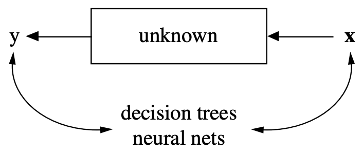
• Both aim to make predictions of natural phenomena:

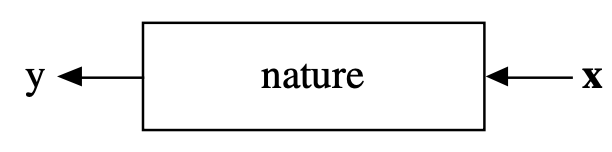
• Statistics:

  • Help humans understand the world

  • Assume data is generated according to an understandable model

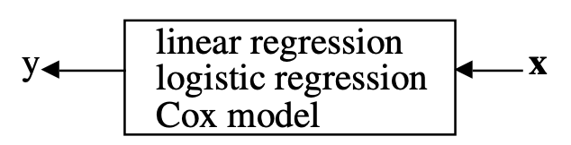
• Machine learning:

  • Automate a task entirely (partially replace the human)

  • Assume that the data generation process is unknown

  • Engineering-oriented, less (too little?) mathematical theory

Types of machine learning¶

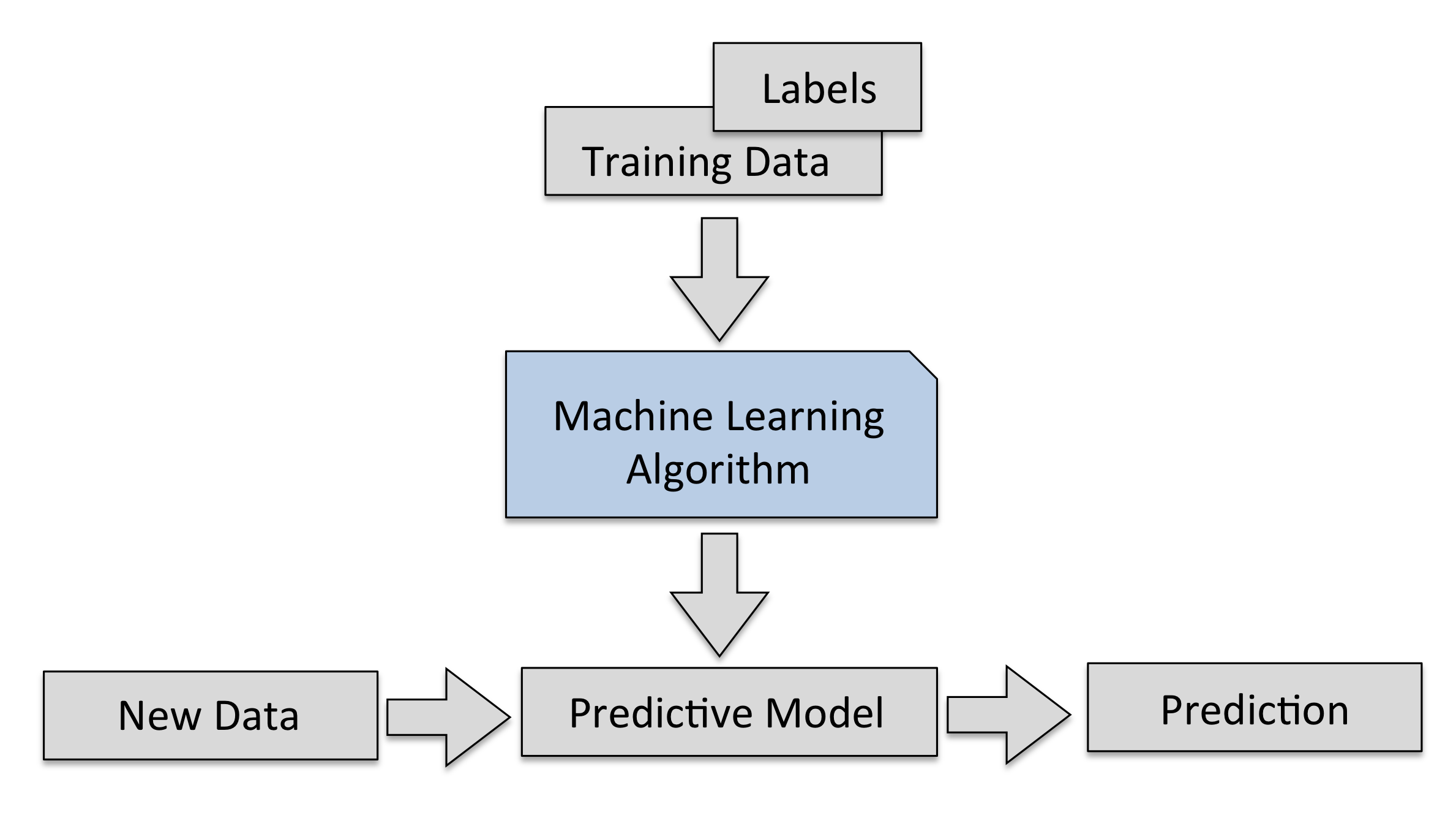
• Supervised Learning: learn a model $f$ from labeled data $(X,y)$ (ground truth)

  • Given a new input X, predict the right output y

  • Given examples of stars and galaxies, identify new objects in the sky

• Unsupervised Learning: explore the structure of the data (X) to extract meaningful information

  • Given inputs X, find which ones are special, similar, anomalous, ...

• Semi-Supervised Learning: learn a model from (few) labeled and (many) unlabeled examples

  • Unlabeled examples add information about which new examples are likely to occur

• Reinforcement Learning: develop an agent that improves its performance based on interactions with the environment

Note: Practical ML systems can combine many types in one system.

Supervised Machine Learning¶

• Learn a model from labeled training data, then make predictions

• Supervised: we know the correct/desired outcome (label)

• Subtypes: classification (predict a class) and regression (predict a numeric value)

• Most supervised algorithms that we will see can do both

Classification¶

• Predict a class label (category), discrete and unordered

  • Can be binary (e.g. spam/not spam) or multi-class (e.g. letter recognition)

  • Many classifiers can return a confidence per class

• The predictions of the model yield a decision boundary separating the classes

Example: Flower classification¶

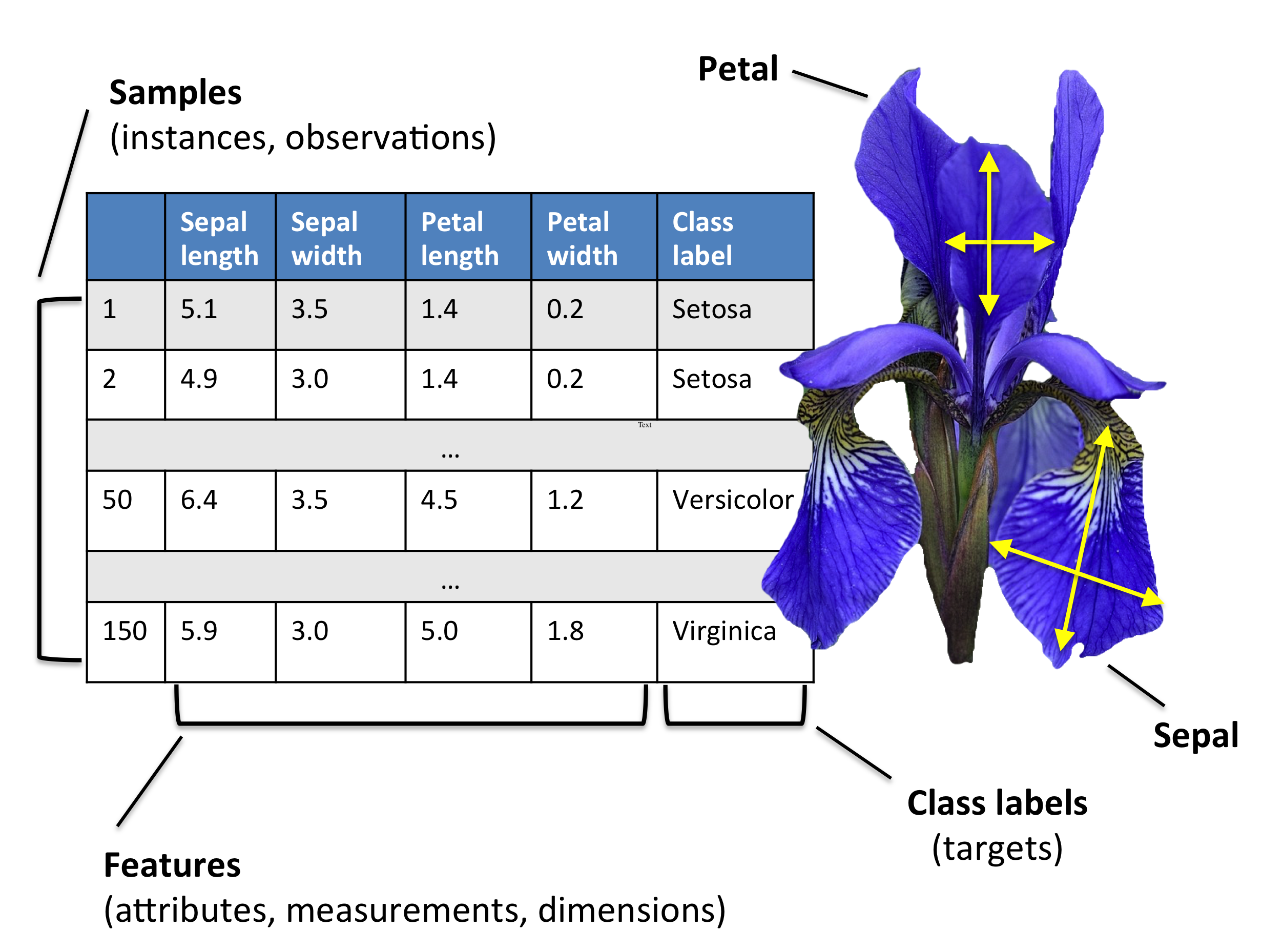
Classify types of Iris flowers (setosa, versicolor, or virginica). How would you do it?

Representation: input features and labels¶

• We could take pictures and use them (pixel values) as inputs (-> Deep Learning)

• We can manually define a number of input features (variables), e.g. length and width of leaves

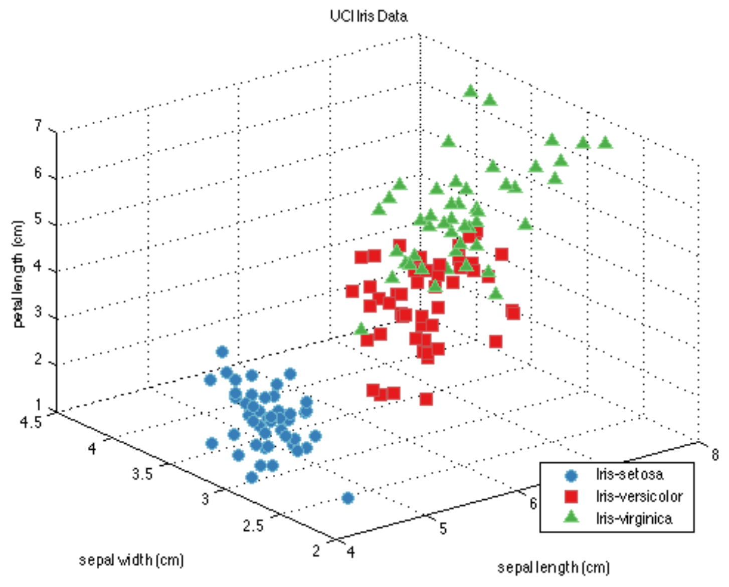
• Every `example’ is a point in a (possibly high-dimensional) space

Regression¶

• Predict a continuous value, e.g. temperature

  • Target variable is numeric

  • Some algorithms can return a confidence interval

• Find the relationship between predictors and the target.

Unsupervised Machine Learning¶

• Unlabeled data, or data with unknown structure

• Explore the structure of the data to extract information

• Many types, we’ll just discuss two.

Clustering¶

• Organize information into meaningful subgroups (clusters)

• Objects in cluster share certain degree of similarity (and dissimilarity to other clusters)

• Example: distinguish different types of customers

Dimensionality reduction¶

• Data can be very high-dimensional and difficult to understand, learn from, store,...

• Dimensionality reduction can compress the data into fewer dimensions, while retaining most of the information

• Contrary to feature selection, the new features lose their (original) meaning

• The new representation can be a lot easier to model (and visualize)

Reinforcement learning¶

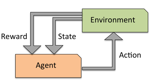
• Develop an agent that improves its performance based on interactions with the environment

  • Example: games like Chess, Go,...

• Search a (large) space of actions and states

• Reward function defines how well a (series of) actions works

• Learn a series of actions (policy) that maximizes reward through exploration

Learning = Representation + Evaluation + Optimization¶

All machine learning algorithms consist of 3 components:

• Representation: A model $f_\theta$ must be represented in a formal language the computer can handle

  • Defines the “concepts” it can learn, the hypothesis space $\mathcal{H}$

  • E.g. decision trees, neural networks, instance-based (k-NN), linear models

• Evaluation: An internal way to choose one hypothesis over another

  • A loss function $\mathcal{L}(f_\theta(X), y)$ that we minimize (often with a regularizer: $\mathcal{L} + \lambda R(\theta)$)

  • Distinct from the task metric $\mathcal{E}$ (e.g. accuracy, F1) we report

  • E.g. difference between correct output $y$ and prediction $\hat{y}$

• Optimization: An efficient way to search the hypothesis space

  • Strategies vary: convex optimization (linear, SVM), greedy growing (trees, boosting), gradient descent (neural nets), lazy / no optimization (k-NN)

  • Start from an initial hypothesis and refine it (or grow it step by step)

  • Many methods, differing in speed, number of optima, and guarantees

• A powerful model is only useful if it can be represented, evaluated, and optimized efficiently — the three components must be balanced.

Neural networks: representation¶

Let’s take neural networks as an example

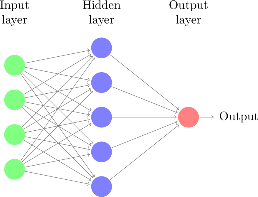
• Representation: a (layered) neural network $f_{\theta}$

  • Each connection has a weight $\theta_i$ (a.k.a. model parameters)

  • Each node receives weighted inputs, applies a nonlinear activation, emits a new value

  • The model $f_\theta$ returns the output of the last layer

• The architecture (number of layers, number/type of neurons) is fixed

  • We call these hyperparameters (set by the user, fixed during training)

Neural networks: evaluation and optimization¶

• Representation: given the structure, the model is fully described by its parameters $\theta$

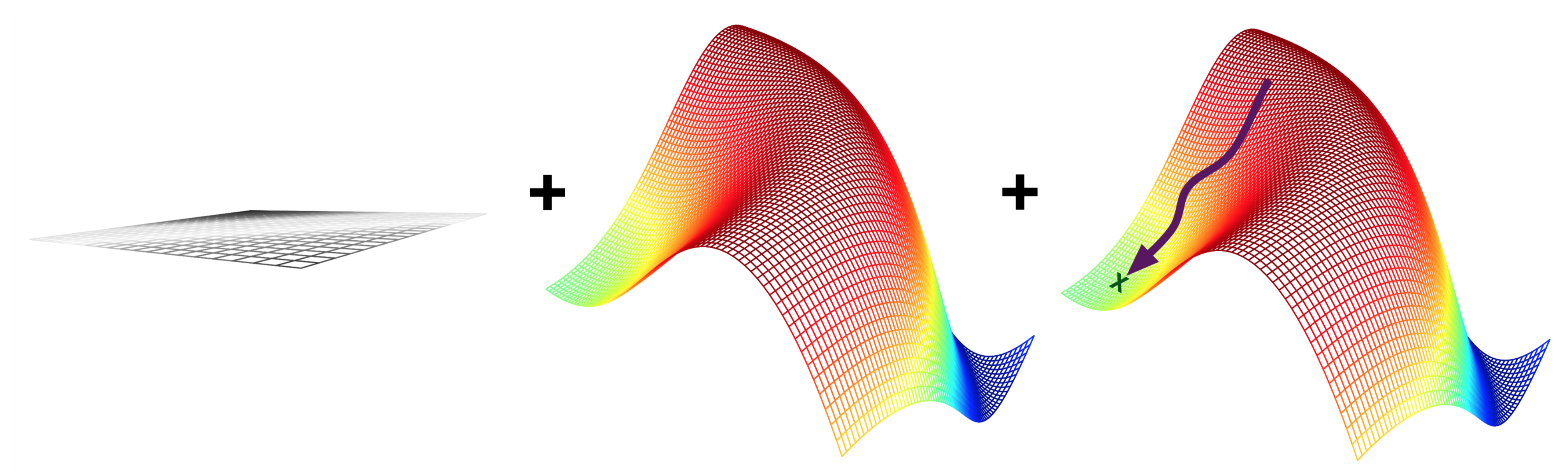
  • Imagine a mini-net with two weights $(\theta_0, \theta_1)$: a 2-dimensional search space

• Evaluation: a loss function $\mathcal{L}(f_\theta(X), y)$ measures how well the predictions match the targets

  • Estimated on a set of training data with the “correct” predictions

  • We cannot see the full loss surface — we can only evaluate specific sets of parameters

• Optimization: find the parameter set $\theta^*$ that minimizes $\mathcal{L}$

  • Usually a type of search in the hypothesis space

  • E.g. gradient descent (simultaneous update of all parameters):

    $$\theta_i \leftarrow \theta_i - \eta \, \frac{\partial \mathcal{L}}{\partial \theta_i}, \quad \forall i$$

    (5)

Overfitting and Underfitting¶

• It’s easy to build a complex model that is 100% accurate on the training data, but very bad on new data

• Overfitting: building a model that is too complex for the amount of data you have

  • You model peculiarities in your training data (noise, biases,...)

  • Solve by making model simpler (regularization), or getting more data

  • Most algorithms have hyperparameters that allow regularization

• Underfitting: building a model that is too simple given the complexity of the data

  • Use a more complex model

• There are techniques for detecting overfitting (e.g. bias-variance analysis). More about that later

• You can build ensembles of many models to overcome both underfitting and overfitting

• There is often a sweet spot that you need to find by optimizing the choice of algorithms and hyperparameters, or using more data.

• Example: regression using polynomial functions

Model selection¶

• Next to the (internal) loss function, we need an (external) evaluation function

  • Feedback signal: are we actually learning the right thing?

    • Are we under/overfitting?

  • Carefully choose to fit the application.

  • Needed to select between models (and hyperparameter settings)

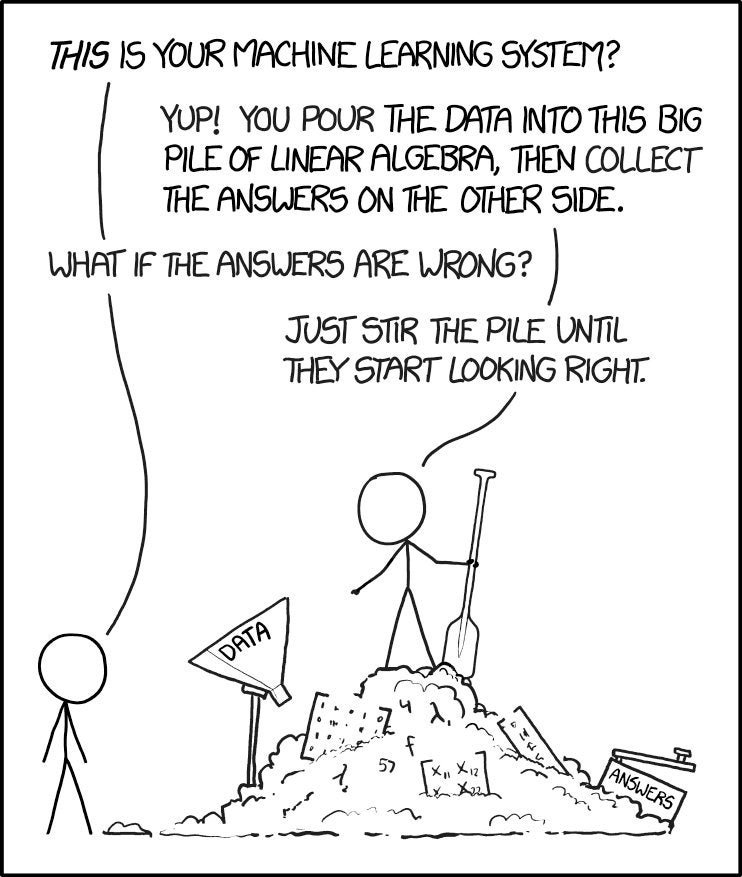
© XKCD

• Data needs to be split into training and test sets

  • Optimize model parameters on the training set, evaluate on independent test set

• Avoid data leakage:

  • Never optimize hyperparameter settings on the test data

  • Never choose preprocessing techniques based on the test data

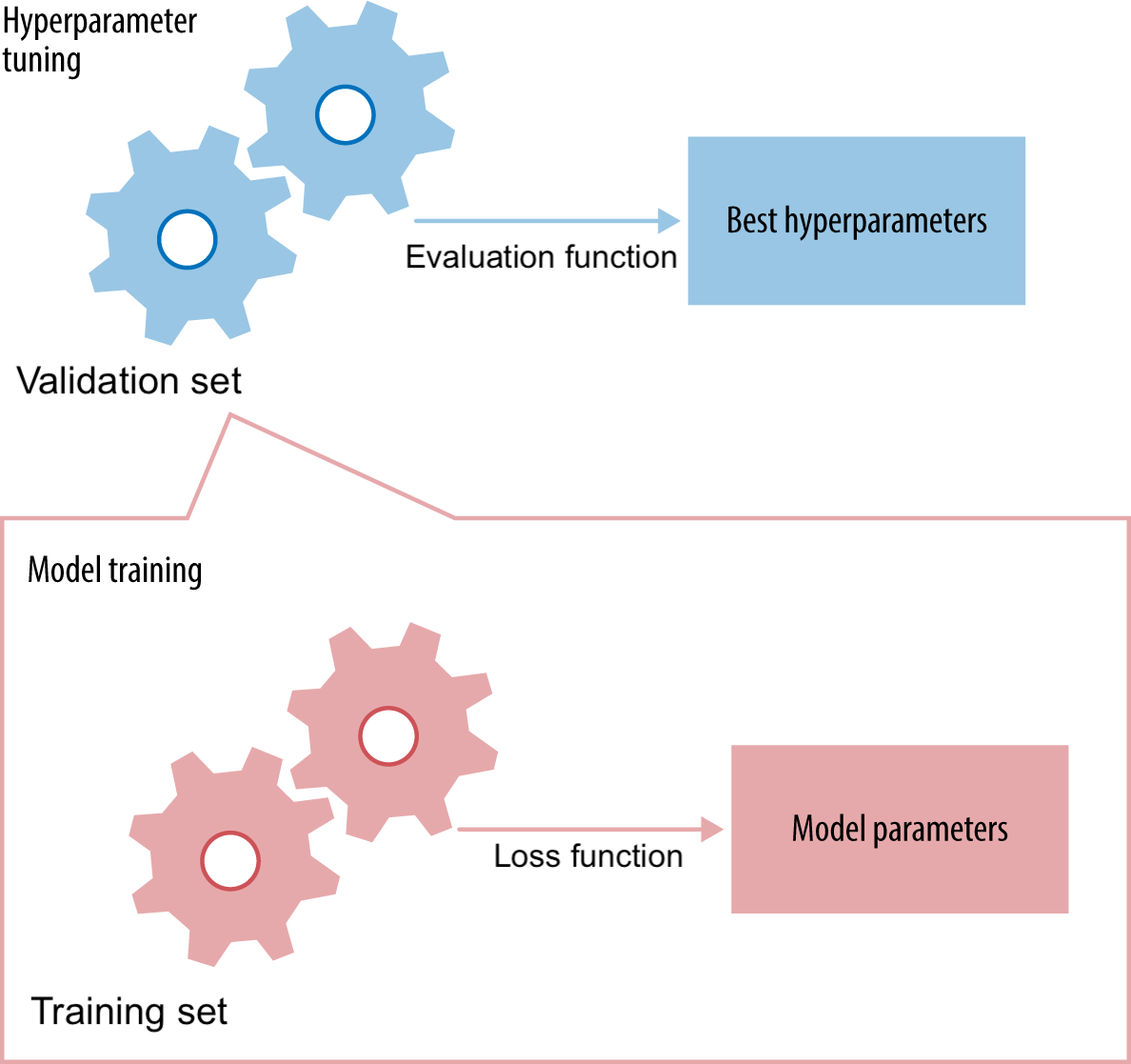
• To optimize hyperparameters and preprocessing as well, set aside part of training set as a validation set

  • Keep test set hidden during all training

• For a given hyperparameter setting, learn the model parameters on training set

  • Minize the loss

• Evaluate the trained model on the validation set

  • Tune the hyperparameters to maximize a certain metric (e.g. accuracy)

Only generalization counts!¶

• Never evaluate your final models on the training data, except for:

  • Tracking whether the optimizer converges (learning curves)

  • Diagnosing under/overfitting:

    • Low training and test score: underfitting

    • High training score, low test score: overfitting

• Always keep a completely independent test set

• On small datasets, use multiple train-test splits to avoid sampling bias

  • You could sample an ‘easy’ test set by accident

  • E.g. Use cross-validation (see later)

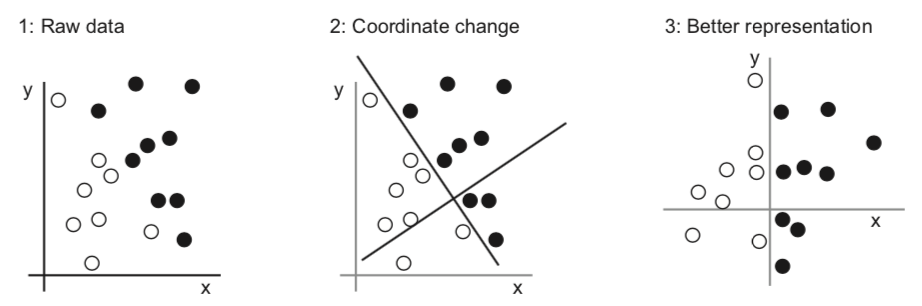
Better data representations, better models¶

• Algorithm needs to correctly transform the inputs to the right outputs

• A lot depends on how we present the data to the algorithm

  • Transform data to better representation (a.k.a. encoding or embedding)

  • Can be done end-to-end (e.g. deep learning) or by first ‘preprocessing’ the data (e.g. feature selection/generation)

Feature engineering¶

• Most machine learning techniques require humans to build a good representation of the data

• Especially when data is naturally structured (e.g. table with meaningful columns)

• Feature engineering is often still necessary to get the best results

  • Feature selection, dimensionality reduction, scaling, ...

  • Applied machine learning is basically feature engineering (Andrew Ng)

• Nothing beats domain knowledge (when available) to get a good representation

  • E.g. Iris data: leaf length/width separate the classes well

Build prototypes early-on

Learning data transformations end-to-end¶

• For unstructured data (e.g. images, text), it’s hard to extract good features

• Deep learning: learn your own representation (embedding) of the data

  • Through multiple layers of representation (e.g. layers of neurons)

  • Each layer transforms the data a bit, based on what reduces the error

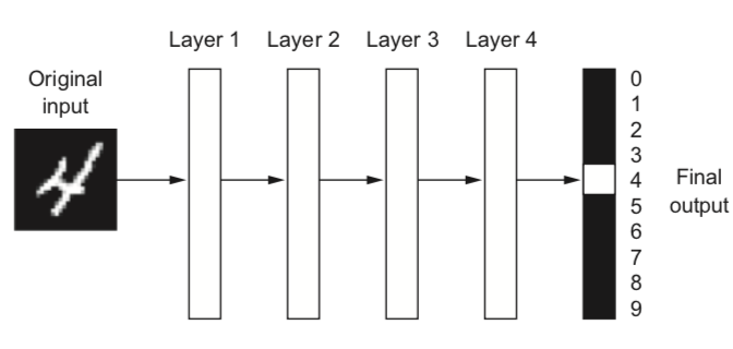
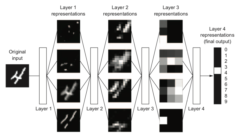
Example: digit classification¶

• Input pixels go in, each layer transforms them to an increasingly informative representation for the given task

• Often less intuitive for humans

Curse of dimensionality¶

• Just adding lots of features and letting the model figure it out doesn’t work

• Our assumptions (inductive biases) often fail in high dimensions:

  • Randomly sample points in an n-dimensional space (e.g. a unit hypercube)

  • Almost all points become outliers at the edge of the space

  • Distances between any two points will become almost identical

Practical consequences¶

• For every dimension (feature) you add, you need exponentially more data to avoid sparseness

• Affects any algorithm that is based on distances (e.g. kNN, SVM, kernel-based methods, tree-based methods,...)

• Blessing of non-uniformity: on many applications, the data lives in a very small subspace

  • You can drastically improve performance by selecting features or using lower-dimensional data representations

“More data can beat a cleverer algorithm”¶

(but you need both)

• More representative data reduces the chance of overfitting

• More data mitigates the curse of dimensionality: the same number of points become denser in a high-dimensional feature space

• Non-parametric models: effective number of parameters grows with data

  • Tree-based methods, k-Nearest Neighbors, kernel methods, ...

  • Universal approximators: can fit increasingly complex functions given sufficient data

• Parametric (fixed-size) models: fixed number of model parameters

  • Linear models, fixed-architecture Neural Networks, ...

  • Capacity can be scaled up (millions of weights) to benefit from more data

  • Deep networks can approximate almost any function, but training may suffer from local minima / non-convex optimization

• Algorithms still matter: a better inductive bias (assumptions matched to the data’s structure) yields higher sample efficiency — the model reaches the same accuracy with less data. This is why CNNs beat MLPs on images, and why pretraining transfers useful biases to data-scarce tasks.

• The bottleneck shifts from data to compute/scalability

Building machine learning systems¶

A typical machine learning system has multiple components, which we will cover in upcoming lectures:

• Preprocessing: Raw data is rarely ideal for learning

  • Feature scaling: bring values in same range

  • Encoding: make categorical features numeric

  • Discretization: make numeric features categorical

  • Label imbalance correction (e.g. downsampling)

  • Feature selection: remove uninteresting/correlated features

  • Dimensionality reduction can also make data easier to learn

  • Using pre-learned embeddings (e.g. word-to-vector, image-to-vector)

• Learning and evaluation

  • Every algorithm has its own biases

  • No single algorithm is always best

  • Model selection compares and selects the best models

    • Different algorithms, different hyperparameter settings

  • Split data in training, validation, and test sets

• Prediction

  • Final optimized model can be used for prediction

  • Expected performance is performance measured on independent test set

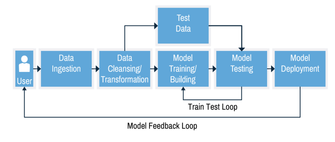
• Together they form a workflow or pipeline

  • Pipeline = linear, automated chain (e.g., sklearn Pipeline)

  • Workflow = broader lifecycle incl. humans, versioning, monitoring

• AutoML exists to build and tune these pipelines

  • CASH problem (Combined Algorithm Selection & Hyperparameter optimization)

  • Methods: Bayesian optimization, Hyperband, NAS, pipeline synthesis (TPOT)

  • AutoML scales expertise; it does not replace it

• You need to optimize pipelines continuously — a model is never “done”

  • Concept drift: P(Y|X) changes over time (sudden / gradual / recurring)

    • Distinct from covariate shift (only P(X) changes)

  • Feedback loops: predictions shape future data (performative prediction)

    • Self-reinforcing loops (recommenders, predictive policing, medical) → bias amplification

    • Mitigation: A/B testing, exploration, counterfactual evaluation

Summary¶

• Learning algorithms contain 3 components:

  • Representation: a model $f_\theta$ mapping input $X$ to predictions $\hat{y}$

    • Model parameters $\theta$ are fit to the data

  • Loss function $\mathcal{L}(f_\theta(X), y)$: measures how well predictions match targets

  • Optimization: $\theta^* = \underset{\theta}{\operatorname{argmin}} \; \mathcal{L}(f_\theta(X), y)$

• Model selection is a bilevel problem:

  • Inner loop: fit $\theta$ on training data $\theta^*(b) = \underset{\theta}{\operatorname{argmin}} \; \mathcal{L}_{\text{train}}(f_{\theta,b}(X_{\text{train}}), y_{\text{train}})$

  • Outer loop: select hyperparameters $b$ on validation data $b^* = \underset{b}{\operatorname{argmin}} \; \mathcal{E}_{\text{val}}(f_{\theta^*(b),b}(X_{\text{val}}), y_{\text{val}})$

  • Inductive bias: assumptions about the model class (linearity, locality, equivariance); hyperparameters control capacity within that class

  • $\mathcal{L}$ is the (differentiable) surrogate we optimize; $\mathcal{E}$ is the task metric we report (e.g., accuracy)

• Overfitting: low training error, high test error

  • Split into (multiple) train-validation-test splits; touch test set only once

  • Regularization (L1/L2, dropout, early stopping): penalizes complexity; its strength is a hyperparameter tuned on validation

  • More data, data augmentation, feature selection, ensembles

• Underfitting: high training and test error — model too simple; increase capacity or improve features

• Machine learning pipelines: preprocessing + learning + deployment + monitoring