Bias-Variance Tradeoff

Bias-Variance Tradeoff
Mahmood Amintoosi, Fall 2025
Computer Science Dept, Ferdowsi University of Mashhad
Further Reading
import numpy as np
from numpy import polyfit
from numpy import polyval
import matplotlib.pyplot as plt
from collections import defaultdict
def f(x):
return np.sin(x * np.pi)def error_function(pred, actual):
return (pred - actual) ** 2np.random.seed(120)
n_observations_per_dataset = 25
n_datasets = 1000
max_poly_degree = 12 # Maximum model complexity
model_poly_degrees = range(1, max_poly_degree + 1)NOISE_STD = .5
percent_train = .8
n_train = int(np.ceil(n_observations_per_dataset * percent_train))x = np.linspace(-1, 1, n_observations_per_dataset)
x = np.random.permutation(x)
x_train = x[:n_train]
x_test = x[n_train:]theta_hat = defaultdict(list)
pred_train = defaultdict(list)
pred_test = defaultdict(list)
train_errors = defaultdict(list)
test_errors = defaultdict(list)for dataset in range(n_datasets):
# Simulate training/testing targets
y_train = f(x_train) + NOISE_STD * np.random.randn(*x_train.shape)
y_test = f(x_test) + NOISE_STD * np.random.randn(*x_test.shape)
# Loop over model complexities
for degree in model_poly_degrees:
# Train model
tmp_theta_hat = polyfit(x_train, y_train, degree)
# Make predictions on train set
tmp_pred_train = polyval(tmp_theta_hat, x_train)
pred_train[degree].append(tmp_pred_train)
# Test predictions
tmp_pred_test = polyval(tmp_theta_hat, x_test)
pred_test[degree].append(tmp_pred_test)
# Mean Squared Error for train and test sets
train_errors[degree].append(np.mean(error_function(tmp_pred_train, y_train)))
test_errors[degree].append(np.mean(error_function(tmp_pred_test, y_test)))# Visualization
plt.figure(figsize=(12, 10))
# Loop through each model complexity for visualization
for degree in model_poly_degrees:
plt.subplot(4, 3, model_poly_degrees.index(degree) + 1)
# Plot training data
plt.scatter(x_train, y_train, color='blue', label='Training Data', alpha=0.5)
plt.scatter(x_test, y_test, color='orange', label='Testing Data', alpha=0.5)
# Plot predictions for the last dataset
# Sort the data for plotting
sorted_indices_train = np.argsort(x_train)
# Plot predictions for the last dataset using sorted data
plt.plot(x_train[sorted_indices_train], pred_train[degree][-1][sorted_indices_train], label='Train Prediction', color='green')
plt.scatter(x_test, pred_test[degree][-1], label='Test Prediction', color='red')
# Plot the true function
x_fine = np.linspace(-1, 1, 100)
plt.plot(x_fine, f(x_fine), 'k--', label='True Function')
plt.title(f'Polynomial Degree {degree}')
plt.xlabel('x')
plt.ylabel('y')
plt.ylim([-2, 2])
plt.legend()
plt.grid()
plt.tight_layout()
plt.show()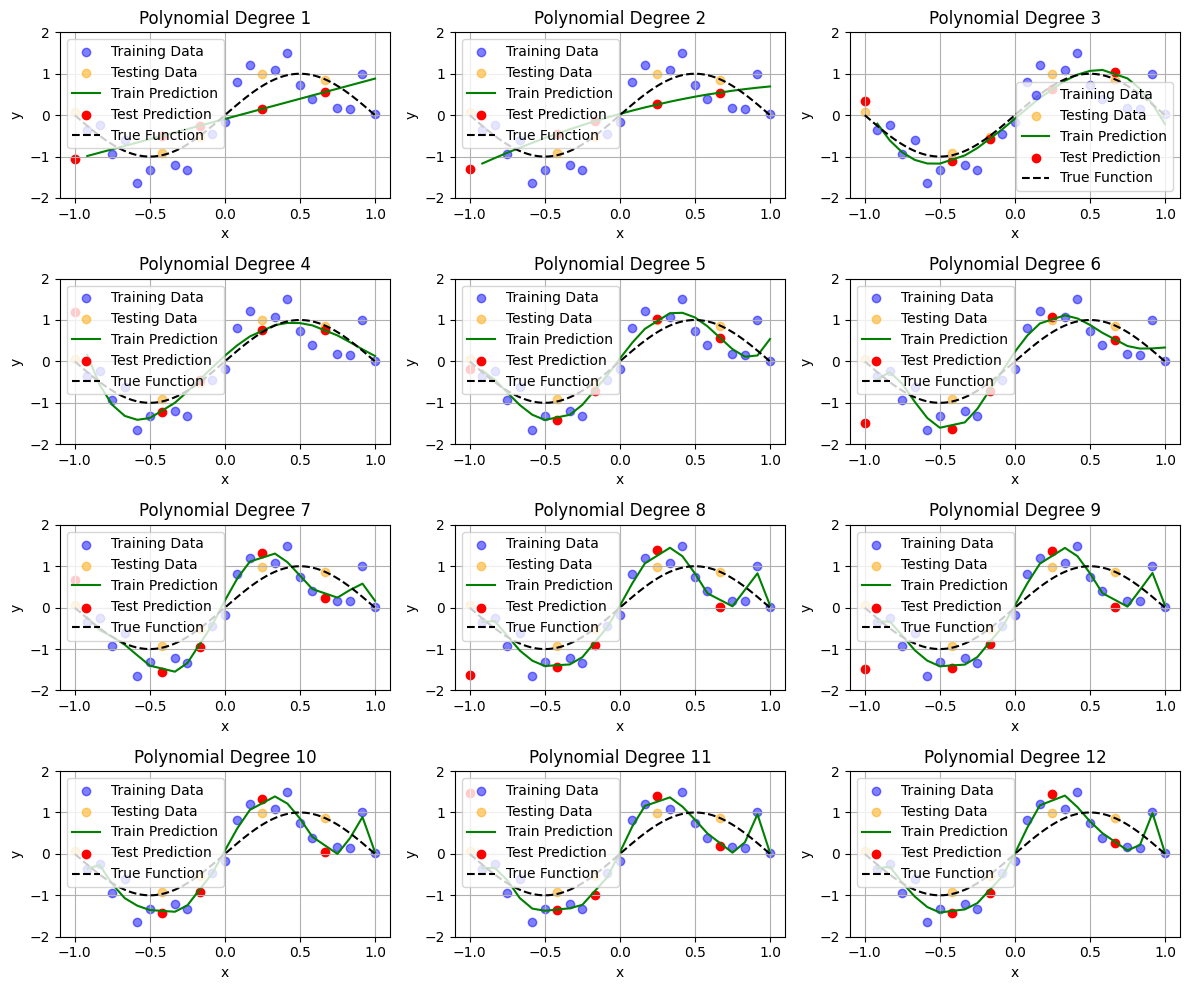
def calculate_estimator_bias_squared(pred_test):
    pred_test = np.array(pred_test)
    average_model_prediction = pred_test.mean(0)

    return np.mean((average_model_prediction - f(x_test)) ** 2)
def calculate_estimator_variance(pred_test):
pred_test = np.array(pred_test)
average_model_prediction = pred_test.mean(0)
return np.mean((pred_test - average_model_prediction) ** 2)complexity_train_error = []
complexity_test_error = []
bias_squared = []
variance = []
for degree in model_poly_degrees:
complexity_train_error.append(np.mean(train_errors[degree]))
complexity_test_error.append(np.mean(test_errors[degree]))
bias_squared.append(calculate_estimator_bias_squared(pred_test[degree]))
variance.append(calculate_estimator_variance(pred_test[degree]))
best_model_degree = model_poly_degrees[np.argmin(complexity_test_error)]
plt.figure(figsize=(5, 3))
plt.plot(model_poly_degrees, bias_squared, color='blue', label='$bias^2$', linewidth=5)
plt.plot(model_poly_degrees, variance, color='green', label='variance', linewidth=5)
plt.plot(model_poly_degrees, np.array(bias_squared) + np.array(variance), linewidth=3, color='black', label='Total Error')
plt.axvline(best_model_degree, color='black', linestyle='--', linewidth=2, label=f'Optimal Model Complexity (Degree={best_model_degree})')

plt.xlabel('Model Complexity (Polynomial Degree)')
plt.ylabel('Error')
plt.ylim([0, .25])
plt.xlim([2, 6])
plt.legend()
plt.title('Bias-Variance Tradeoff')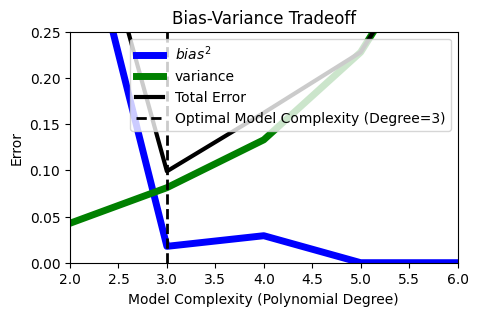
Notebook Cell
# # https://spotintelligence.com/2023/04/11/bias-variance-trade-off/
# from sklearn.model_selection import train_test_split
# from sklearn.preprocessing import PolynomialFeatures
# from sklearn.linear_model import LinearRegression
# from sklearn.metrics import mean_squared_error
# import matplotlib.pyplot as plt
# import numpy as np

# # Generate some synthetic data with a non-linear relationship
# np.random.seed(0)
# x = np.linspace(-5, 5, num=100)
# # y = x ** 3 + np.random.normal(size=100)
# y = f(x) #np.sin(x * np.pi)

# # Split the data into training and testing sets
# x_train, x_test, y_train, y_test = train_test_split(x, y, test_size=0.2, random_state=0)

# # Fit polynomial regression models with different degrees of polynomials
# degrees = [1, 2, 3, 4, 5, 8, 10]
# train_errors, test_errors = [], []
# bias_squared = []
# variance = []

# for degree in degrees:

#     # Transform the features to polynomial features
#     poly_features = PolynomialFeatures(degree=degree)
#     x_poly_train = poly_features.fit_transform(x_train.reshape(-1, 1))
#     x_poly_test = poly_features.transform(x_test.reshape(-1, 1))

#     # Fit the linear regression model to the polynomial features
#     model = LinearRegression()
#     model.fit(x_poly_train, y_train)

#     # Evaluate the model on the training and testing data
#     y_pred_train = model.predict(x_poly_train)
#     y_pred_test = model.predict(x_poly_test)
#     train_error = mean_squared_error(y_train, y_pred_train)
#     test_error = mean_squared_error(y_test, y_pred_test)
#     train_errors.append(train_error)
#     test_errors.append(test_error)
#     bias_squared.append(calculate_estimator_bias_squared(y_pred_test))
#     variance.append(calculate_estimator_variance(y_pred_test))


# # Plot the training and testing errors as a function of the degree of polynomial

# plt.plot(degrees, train_errors, label='Training error')
# plt.plot(degrees, test_errors, label='Testing error')
# plt.plot(degrees, bias_squared, color='blue', label='$bias^2$', linewidth=5)
# plt.plot(degrees, variance, color='green', label='variance', linewidth=5)

# plt.legend()
# plt.xlabel('Degree of polynomial')
# plt.ylabel('Mean squared error')
# plt.show()