High-Dimensional Data and the Curse of Dimensionality
Mahmood Amintoosi, Fall 2026
Computer Science Dept, Ferdowsi University of Mashhad
The geometric facts on this page are those of The Elements of Statistical Learning (Hastie et al. (2009)), §2.5, and chapter 6 of Zaki’s Data Mining and Machine Learning (Zaki & Meira (2020)).
Learning objectives. By the end you should be able to
compute the volume of a ball and of a cube in dimensions and explain why their ratio tends to zero;
explain why a neighbourhood containing a fixed fraction of the data is not local in high dimensions, and compute its edge length ;
show that in high dimension the nearest and the farthest neighbour are almost equally far away, and say what that does to k-NN;
explain why most of the volume of a ball is in a thin shell, and why Gaussian samples concentrate at radius ;
sample points uniformly inside a ball and on its surface (why the naive radius is wrong);
measure the effect of the dimension on a k-NN classifier, with and without more data.
Introduction¶
In modern data mining and machine learning we often deal with data in very high-dimensional spaces (images, text embeddings, genomic data). A dataset is typically represented as an matrix : points, features.
High-dimensional space, or hyperspace, does not behave like the geometry of two or three dimensions. The collection of effects that follow from this is called the curse of dimensionality. The five phenomena we look at are:
Volume concentration: the volume of a hypersphere vanishes relative to the hypercube that contains it.
The problem of local neighborhoods: a “local” neighbourhood of a fixed fraction of the data is not local any more, so methods such as k-NN lose their meaning (ESL §2.5).
Distance concentration: the nearest and the farthest neighbour are almost at the same distance, so ranking neighbours becomes meaningless.
The thin shell: almost all of the volume of a ball sits near its surface.
Orthogonality and Gaussian behaviour: random vectors are nearly orthogonal, and Gaussian samples concentrate in a thin shell at radius .
Throughout, is the number of dimensions. The figures taken from ESL label it ; the text here uses consistently.
import math

import matplotlib.pyplot as plt
import numpy as np

SEED = 42
rng = np.random.default_rng(SEED)


def ball_volume(d, r=1.0):
    """Volume of the d-dimensional ball of radius r: K_d * r^d."""
    return math.pi ** (d / 2) * r ** d / math.gamma(d / 2 + 1)


def shell_volume(d, r=1.0, thickness=0.2):
    """Volume of the shell of the given thickness just inside the surface."""
    return ball_volume(d, r) - ball_volume(d, max(r - thickness, 0.0))


dimensions = range(1, 30)
plt.figure(figsize=(9, 5))
plt.plot(list(dimensions), [ball_volume(d) for d in dimensions], marker="o", ms=4,
         label=r"volume of the unit ball, $K_d$")
plt.plot(list(dimensions), [2.0 ** d for d in dimensions], marker="s", ms=3,
         label=r"volume of the cube $[-1,1]^d$, $2^d$")
plt.yscale("log")
plt.xlabel("dimension $d$")
plt.ylabel("volume (log scale)")
plt.title("The ball grows, the cube explodes")
plt.legend(frameon=False)
plt.grid(alpha=0.3)
plt.show()

for d in [1, 2, 3, 10, 20]:
    print(f"d = {d:2d}:  ball volume = {ball_volume(d):.3e}   "
          f"ratio ball/cube = {ball_volume(d) / 2 ** d:.3e}")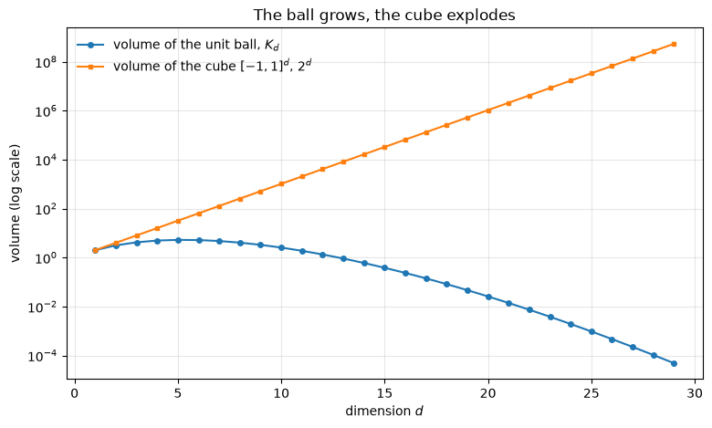
d =  1:  ball volume = 2.000e+00   ratio ball/cube = 1.000e+00
d =  2:  ball volume = 3.142e+00   ratio ball/cube = 7.854e-01
d =  3:  ball volume = 4.189e+00   ratio ball/cube = 5.236e-01
d = 10:  ball volume = 2.550e+00   ratio ball/cube = 2.490e-03
d = 20:  ball volume = 2.581e-02   ratio ball/cube = 2.461e-08
Geometry of Hyperspace: Cubes and Balls¶
The Hypercube¶
The data space is often taken as a -dimensional hypercube. For a hypercube of side length the volume is simply
The Ball and the Sphere¶
Two different objects are needed, and confusing them is a classic source of errors:
the ball is the solid; its volume is
the sphere is only the surface — a set of measure zero — and is written with because it is a -dimensional object living in . Its area is , the derivative of the volume with respect to .
is the Gamma function; for integer arguments .
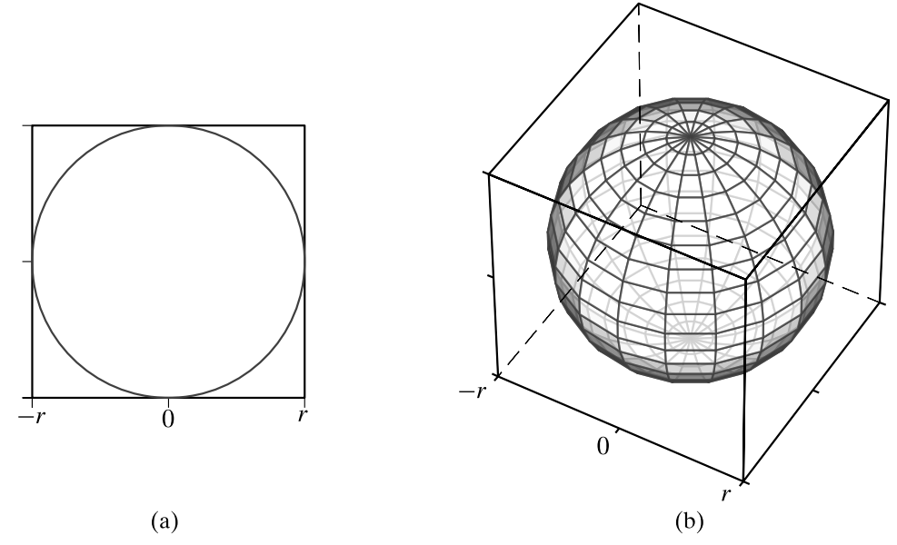
Figure 6.4. A hypersphere inscribed in a hypercube: (a) two and (b) three dimensions (Zaki, ch. 6).
The Empty Center (the “Porcupine” Effect)¶
Take the largest ball that fits inside a cube of side , that is . The ratio of their volumes is
Implication. As the dimension grows, the ball becomes negligible compared with the cube: almost all of the volume of the cube is in its corners, and the center is essentially empty. In dimensions there are corners.
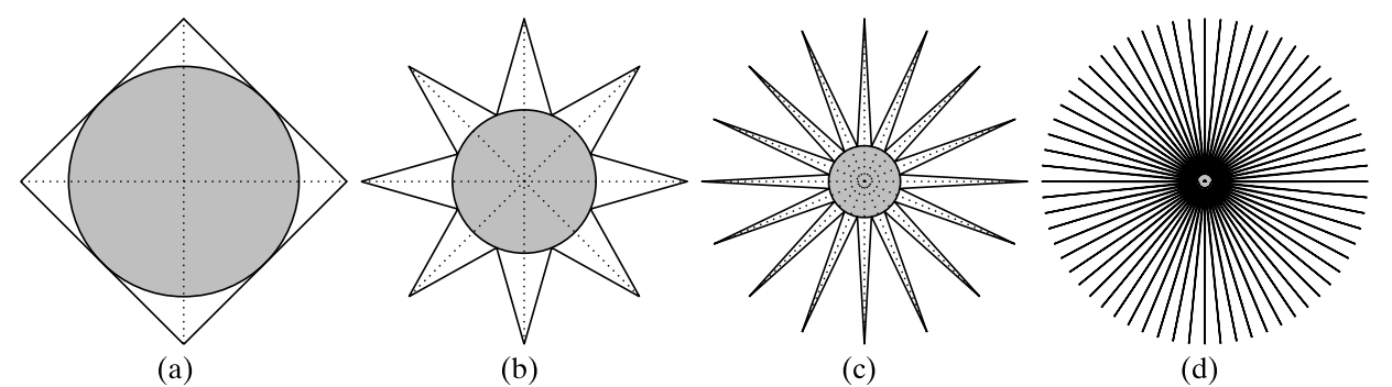
Conceptual view of high-dimensional space: (a) two, (b) three, (c) four and (d) higher dimensions. In dimensions there are corners; the radius of the inscribed ball is what makes the difference between the volume of the cube and of the ball visible (Zaki, ch. 6).
The Problem of Local Neighborhoods¶
One of the most consequential manifestations of the curse of dimensionality is that “local” methods such as k-nearest neighbours stop being local.
The Edge Length of a Neighborhood¶
Suppose the inputs are uniformly distributed in the unit hypercube and we want a neighbourhood that contains a fraction of the observations. That neighbourhood must cover a fraction of the volume, and if it is a subcube of edge length then
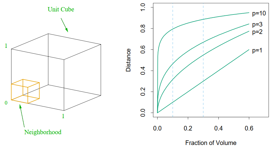
Figure 2.6 (ESL). The side length of the subcube needed to capture a fraction of the volume of the data, for different dimensions (the figure labels the dimension ; here it is ). In ten dimensions we must cover 80% of the range of each coordinate to capture 10% of the data.
def edge_length(fraction, d):
    return fraction ** (1.0 / d)


fractions = np.linspace(0.001, 1.0, 200)
plt.figure(figsize=(7, 5))
for d in [1, 2, 3, 10]:
    plt.plot(fractions, edge_length(fractions, d), label=f"$d={d}$")

plt.plot(0.1, 0.1 ** (1 / 10), "ro")
plt.annotate(r"$d=10,\ r=0.1:\ e_d(r)\approx 0.80$", (0.1, 0.1 ** (1 / 10)),
             xytext=(0.25, 0.62), arrowprops=dict(arrowstyle="->", color="red"))
plt.xlabel(r"fraction of the data, $r$")
plt.ylabel(r"edge length of the subcube, $e_d(r)$")
plt.title("A neighborhood holding 10% of the data")
plt.legend(frameon=False)
plt.grid(alpha=0.3)
plt.show()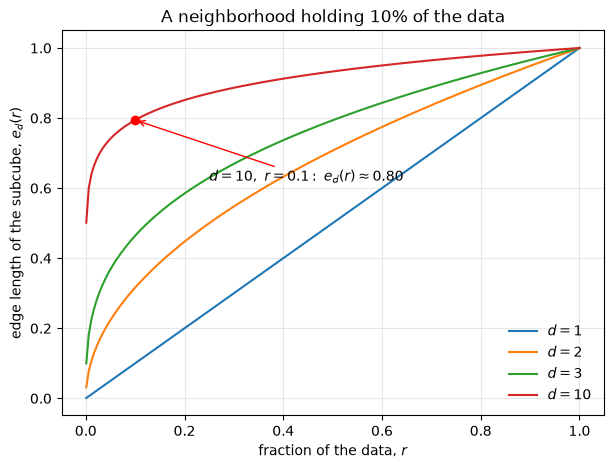
Analysis. With and we need : to capture 10% of the data we must cover 80% of the range of every coordinate. Such a neighbourhood is not local in any useful sense — it is most of the space.
Distance to the Boundary¶
Sampling density is sparse for a second reason. For points drawn uniformly in the unit ball , the median distance from the origin to the closest data point is
Where the formula comes from. The probability that a single uniform point falls in the ball of radius is , so the probability that it falls outside is , and the probability that all points fall outside is . The median of the distance to the closest point is the for which that probability equals :
For and this gives : more than halfway to the boundary. Hence most data points are closer to the boundary of the sample space than to any other data point, and prediction is a problem of extrapolation rather than of interpolation.
Distance Concentration¶
The phenomenon that hurts k-NN most directly is not the edge length but the distances themselves. For a query point, let be the distance to its nearest neighbour and the distance to the farthest point of the sample. In one dimension the ratio is small: there is a genuinely close point. In high dimensions the ratio tends to 1: the closest point is almost as far as the farthest one, so “nearest” is a statement about noise rather than about similarity.
The experiment below draws points uniformly in the unit cube for , takes one random query point, and reports the mean ratio over many queries.
n_points, n_queries = 1000, 50
dims_dc = [2, 10, 100, 1000]
ratios = []

for d in dims_dc:
    data = rng.random((n_points, d))
    queries = rng.random((n_queries, d))
    dist = np.linalg.norm(queries[:, None, :] - data[None, :, :], axis=2)
    ratios.append(np.mean(dist.min(axis=1) / dist.max(axis=1)))

plt.figure(figsize=(7, 4))
plt.plot(dims_dc, ratios, marker="o")
for x, y in zip(dims_dc, ratios):
    plt.annotate(f"{y:.2f}", (x, y), textcoords="offset points", xytext=(0, 8), ha="center")
plt.xscale("log")
plt.xlabel("dimension $d$")
plt.ylabel(r"mean $d_{\min}/d_{\max}$")
plt.title(f"{n_points} uniform points, {n_queries} queries")
plt.ylim(0, 1.05)
plt.grid(alpha=0.3, which="both")
plt.show()

for d, ratio in zip(dims_dc, ratios):
    print(f"d = {d:4d}:  mean d_min/d_max = {ratio:.3f}")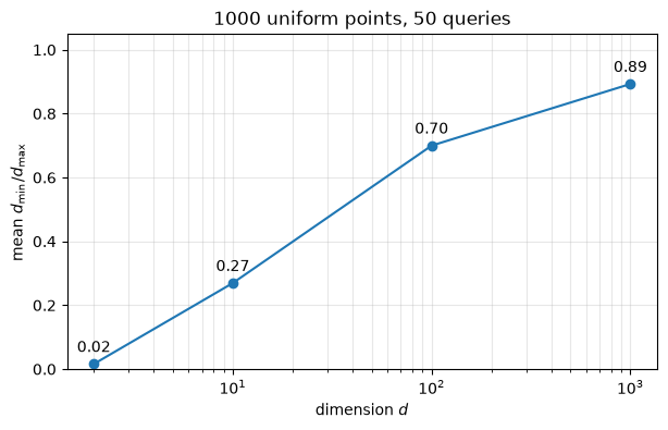
d =    2:  mean d_min/d_max = 0.016
d =   10:  mean d_min/d_max = 0.269
d =  100:  mean d_min/d_max = 0.700
d = 1000:  mean d_min/d_max = 0.893
Read the numbers: in two dimensions the nearest neighbour is typically a small fraction of the farthest distance, so ranking neighbours is informative. In a thousand dimensions the ratio is close to 1 — every point is almost equidistant from every other point. Two consequences:
The neighbour ranking is dominated by noise: which point is “nearest” changes with tiny perturbations of the data, so a k-NN vote is unstable.
A ball around the query that contains neighbours is so large that it contains a good part of the data, so the “local” average is not local.
This is the theoretical reason behind the experiment at the end of this page.
The Thin Shell Argument¶
Where is the volume inside a ball? Consider a thin shell of width just inside the surface of a ball of radius . Its volume is
so the fraction of the volume in the shell is
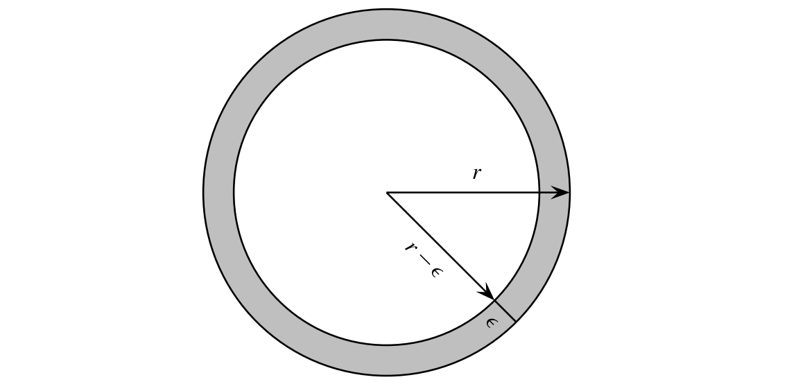
Figure 6.6 (Zaki, ch. 6): the shell of a ball concentrates the volume as grows.
For a disk () with and the shell holds of the area. For the same shell holds — almost two thirds.
Conclusion. In high dimensions, for a shell of fixed relative thickness , almost 100% of the volume — and of the probability mass of a uniform distribution — is concentrated near the surface. The interior is essentially empty.
dims_shell = list(range(1, 30))
fraction = [shell_volume(d, 1.0, 0.2) / ball_volume(d, 1.0) for d in dims_shell]

plt.figure(figsize=(9, 5))
plt.plot(dims_shell, fraction, marker="o", ms=4)
plt.axhline(1.0, color="black", lw=1, ls="--")
plt.xlabel("dimension $d$")
plt.ylabel(r"volume of the shell / volume of the ball")
plt.title(r"Fraction of the volume in a shell of thickness $\epsilon = 0.2\,r$")
plt.grid(alpha=0.3)
plt.show()

for d in [2, 10, 30]:
    print(f"d = {d:2d}:  shell fraction = {shell_volume(d, 1.0, 0.2) / ball_volume(d, 1.0):.3f}")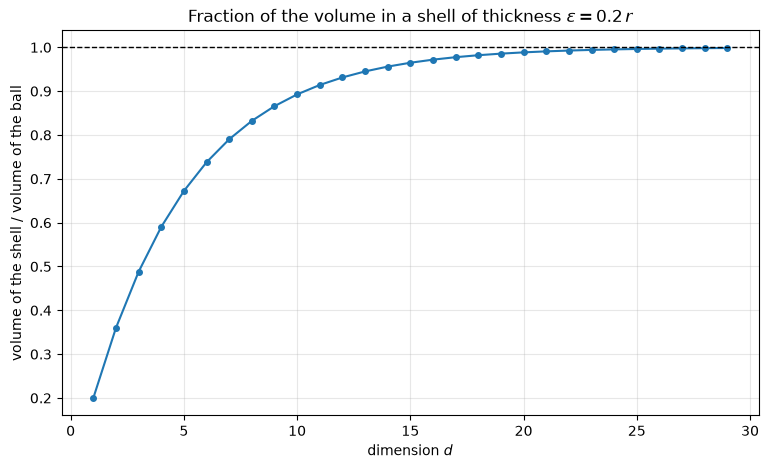
d =  2:  shell fraction = 0.360
d = 10:  shell fraction = 0.893
d = 30:  shell fraction = 0.999
Aside: Sampling Points Uniformly in a Ball¶
Generating points uniformly inside a ball in high dimensions is a good illustration of the volume facts above, and it is needed by many simulation experiments.
Rejection sampling — generate points uniformly in the cube and keep those inside the ball — has an acceptance rate equal to the ratio of the two volumes, which goes to zero (the porcupine effect). Beyond about ten dimensions it is computationally useless. The table below measures the acceptance rate for with 2000 accepted points, and compares it with the theoretical value .
def rejection_rate(num_points, d, batch_size=1000, max_batches=20000):
    """Acceptance rate of rejection sampling: how much of the cube is in the ball?"""
    accepted, generated = 0, 0
    for _ in range(max_batches):
        batch = rng.uniform(-1, 1, (batch_size, d))
        accepted += int(np.sum(np.sum(batch ** 2, axis=1) <= 1.0))
        generated += batch_size
        if accepted >= num_points:
            break
    return accepted / generated


n_points = 2000
dims_rej = list(range(2, 11))
measured, theoretical = [], []

for d in dims_rej:
    measured.append(rejection_rate(n_points, d))
    theoretical.append(ball_volume(d) / 2 ** d)

plt.figure(figsize=(8, 5))
plt.plot(dims_rej, measured, marker="o", label="measured")
plt.plot(dims_rej, theoretical, marker="s", ls="--", label=r"theory: $K_d/2^d$")
plt.yscale("log")
plt.xlabel("dimension $d$")
plt.ylabel("acceptance rate (log scale)")
plt.title(f"rejection sampling from the cube, {n_points} accepted points")
plt.legend(frameon=False)
plt.grid(alpha=0.3, which="both")
plt.show()

for d, m, t in zip(dims_rej, measured, theoretical):
    print(f"d = {d:2d}:  measured = {m:.4f}   theory = {t:.4f}   "
          f"candidates per accepted point = {1 / m:8.1f}")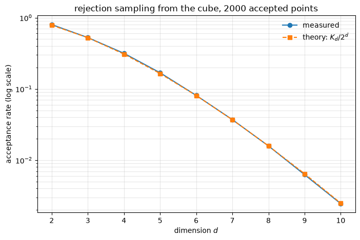
d =  2:  measured = 0.8003   theory = 0.7854   candidates per accepted point =      1.2
d =  3:  measured = 0.5255   theory = 0.5236   candidates per accepted point =      1.9
d =  4:  measured = 0.3163   theory = 0.3084   candidates per accepted point =      3.2
d =  5:  measured = 0.1687   theory = 0.1645   candidates per accepted point =      5.9
d =  6:  measured = 0.0811   theory = 0.0807   candidates per accepted point =     12.3
d =  7:  measured = 0.0371   theory = 0.0369   candidates per accepted point =     27.0
d =  8:  measured = 0.0158   theory = 0.0159   candidates per accepted point =     63.2
d =  9:  measured = 0.0062   theory = 0.0064   candidates per accepted point =    160.0
d = 10:  measured = 0.0025   theory = 0.0025   candidates per accepted point =    408.0
The measured rate falls off geometrically and follows : by only about one candidate point in four hundred lands inside the ball, and the cost per accepted point keeps doubling with every extra dimension.
Points on the Surface: Gaussian Directions¶
The trick that makes uniform sampling easy is to use the spherical symmetry of the Gaussian distribution. If independently, the joint density is
which depends on the length only, never on the direction. The distribution is therefore invariant under rotations (isotropic), all directions are equally likely, and
is uniformly distributed on the unit sphere .
n_dir = 500
d_vis = 2

x = rng.standard_normal((n_dir, d_vis))
y_surface = x / np.linalg.norm(x, axis=1, keepdims=True)

plt.figure(figsize=(5, 5))
plt.scatter(x[:, 0], x[:, 1], s=5, alpha=0.6, label="Gaussian sample")
plt.scatter(y_surface[:, 0], y_surface[:, 1], s=5, label="normalised")
plt.gca().set_aspect("equal")
plt.title("Normalising a Gaussian sample gives the circle")
plt.legend(frameon=False, loc="upper right")
plt.show()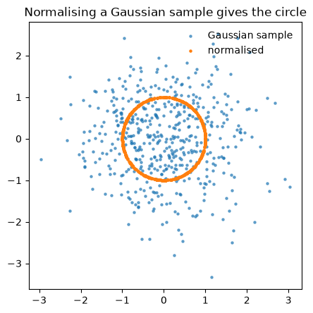
Points Inside the Ball¶
Scaling a direction by a uniform random number is wrong: the volume of a shell at radius grows like , so most of the volume is near the surface and a uniform radius bunches the points near the center.
The right radius. For the uniform distribution inside the ball, the probability that a point lies within radius must be proportional to the volume it encloses:
Inverse transform sampling with then gives . For , :
| 0.00 | 0.10 | 0.25 | 0.50 | 0.75 | 1.00 | |
|---|---|---|---|---|---|---|
| 0.000 | 0.316 | 0.500 | 0.707 | 0.866 | 1.000 |
Algorithm for uniform points in the ball :
draw ;
normalise, — a uniform direction;
draw ;
return .
d_ball = 2
plt.figure(figsize=(11, 5))

for panel, exponent in enumerate([1.0, 1.0 / d_ball]):
    a = rng.random(n_dir)
    rho = a ** exponent
    points = rho[:, None] * y_surface

    plt.subplot(1, 2, panel + 1)
    theta = np.linspace(0, 2 * np.pi, 400)
    plt.plot(np.cos(theta), np.sin(theta), color="black", lw=1)
    plt.scatter(points[:, 0], points[:, 1], s=6)
    plt.gca().set_aspect("equal")
    plt.title(r"$\rho \sim U(0,1)$: bunched at the center" if panel == 0
              else r"$\rho = a^{1/d}$: uniform")
    plt.xlim(-1.1, 1.1)
    plt.ylim(-1.1, 1.1)

plt.tight_layout()
plt.show()

# a quantitative check: the fraction of points inside half the radius must be (1/2)^d
for d in [2, 3, 10]:
    a = rng.random(20000)
    for name, rho in [("naive", a), ("correct", a ** (1 / d))]:
        print(f"d = {d:2d}, {name:7s}: fraction with rho < 0.5 = "
              f"{np.mean(rho < 0.5):.4f}   (expected {(0.5) ** d:.4f})")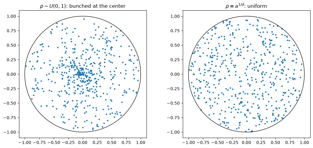
d =  2, naive  : fraction with rho < 0.5 = 0.4967   (expected 0.2500)
d =  2, correct: fraction with rho < 0.5 = 0.2479   (expected 0.2500)
d =  3, naive  : fraction with rho < 0.5 = 0.4966   (expected 0.1250)
d =  3, correct: fraction with rho < 0.5 = 0.1240   (expected 0.1250)
d = 10, naive  : fraction with rho < 0.5 = 0.5015   (expected 0.0010)
d = 10, correct: fraction with rho < 0.5 = 0.0009   (expected 0.0010)
Nearly Orthogonal Directions¶
Another counter-intuitive property is that in high dimensions “every direction is orthogonal to every other one”, or more precisely: random vectors are nearly orthogonal.
The Diagonal of the Hypercube¶
Consider the main diagonal of the cube, . The angle between it and a coordinate axis satisfies
so : the diagonal is almost orthogonal to every axis.
Random Vectors¶
The same holds for two independent random vectors, and the reason is the law of large numbers: for with independent zero-mean, unit-variance entries,
whose numerator is a sum of independent zero-mean terms of variance 1 and therefore of size — the ratio is .
dim = 200
vectors = rng.standard_normal((5, dim))
vectors /= np.linalg.norm(vectors, axis=1, keepdims=True)

cosines = [vectors[i] @ vectors[j]
           for i in range(len(vectors)) for j in range(i + 1, len(vectors))]
print(f"cosine similarities of {len(cosines)} random pairs in {dim}-D:")
print(np.round(cosines, 4))
print(f"max |cosine| = {np.max(np.abs(cosines)):.4f}   (1/sqrt(d) = {1 / np.sqrt(dim):.4f})")
cosine similarities of 10 random pairs in 200-D:
[-0.0401 0.0349 -0.0056 -0.0042 -0.075 -0.0497 -0.0402 0.0836 0.0071
0.1518]
max |cosine| = 0.1518 (1/sqrt(d) = 0.0707)
Gaussian Distribution in High Dimensions¶
From Geometric Shells to Statistical Shells¶
The geometric effects above were about the volume of a ball. The Gaussian distribution shows the same phenomenon statistically: even though its density is maximal at the origin, almost no sample lands near the origin.
Why Gaussian Points Do Not Cluster Near the Mean¶
Let . In one dimension many samples lie “close to zero”, and is usually small. This intuition breaks down from two dimensions on: the density is highest at the origin, but the volume available near the origin is negligible.
In one dimension “the center” is a point and there is no volume growth.
In dimensions the volume of a shell grows like , so the number of points at radius is density volume.
The center has the highest density but almost no volume, so almost no sample lands there.
Distance of a Gaussian Vector from the Origin¶
A single identity explains the behaviour:
So for , for , for and for (see chi-squared distribution). Increasing the dimension pushes all samples outward, not just the outliers: the whole distribution sits in a thin shell around radius .
d_gauss = 200
n_gauss = 5000

x_1d = rng.standard_normal(n_gauss)
norms = np.linalg.norm(rng.standard_normal((n_gauss, d_gauss)), axis=1)

fig, ax = plt.subplots(1, 2, figsize=(11, 4))
ax[0].hist(x_1d, bins=60, color="tab:blue", alpha=0.8)
ax[0].axvline(0, color="red", ls="--", label="mean 0")
ax[0].set_title("1-D Gaussian: mass at the mean")
ax[0].set_xlabel("value")
ax[0].legend(frameon=False)

ax[1].hist(norms, bins=60, color="tab:green", alpha=0.8)
ax[1].axvline(np.sqrt(d_gauss), color="red", ls="--",
              label=rf"$\sqrt{{d}} = {np.sqrt(d_gauss):.1f}$")
ax[1].axvline(0, color="black", lw=1, label="mean 0")
ax[1].set_title(rf"{d_gauss}-D Gaussian: mass at $\sqrt{{d}}$")
ax[1].set_xlabel(r"distance from the origin, $\|\mathbf{x}\|$")
ax[1].legend(frameon=False)
plt.tight_layout()
plt.show()

print(f"mean norm = {norms.mean():.2f}   std = {norms.std():.2f}   sqrt(d) = {np.sqrt(d_gauss):.2f}")
print(f"fraction of samples with norm within 10% of sqrt(d): "
      f"{np.mean(np.abs(norms - np.sqrt(d_gauss)) < 0.1 * np.sqrt(d_gauss)):.2f}")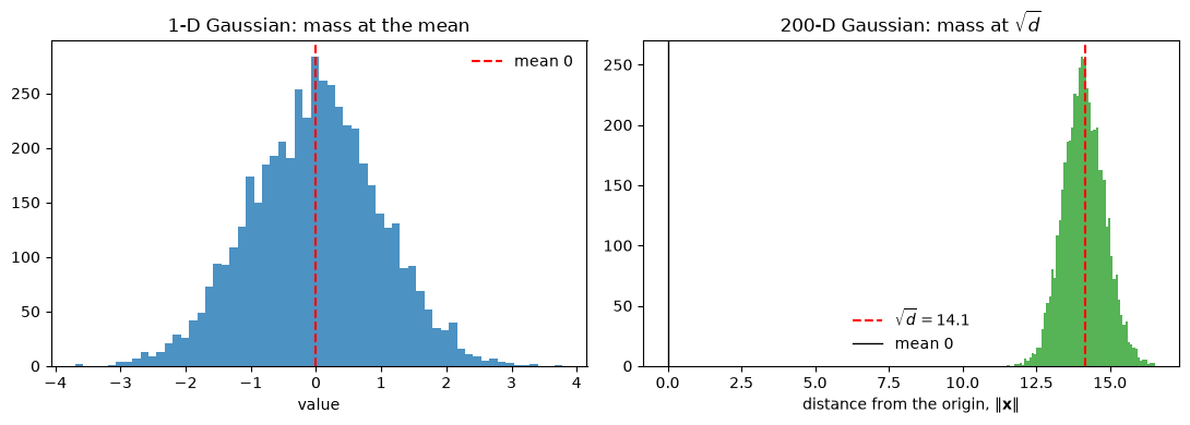
mean norm = 14.12   std = 0.70   sqrt(d) = 14.14
fraction of samples with norm within 10% of sqrt(d): 0.96
The two histograms are the statistical version of the geometric thin-shell effect: one- dimensional Gaussian data sit at the mean, two-hundred-dimensional Gaussian data sit on a sphere of radius 14.1 with a width that does not grow with .
The Gaussian Annulus Phenomenon¶
The formal statement is:
With overwhelming probability a Gaussian sample lies within of the origin — a thin annulus whose thickness does not grow with .
As increases the radius grows like while the thickness stays constant, so the relative thickness tends to zero. This is the reason Gaussian vectors are used in theory: they are the geometry of high-dimensional space, in the same way that uniform points in a ball are.
Connection with the Previous Sections¶
| earlier result | Gaussian version |
|---|---|
| the center of the ball is empty | Gaussian mass avoids the origin |
| uniform volume concentrates at the surface | Gaussian mass concentrates at |
| uniform sampling needs | Gaussian sampling does this automatically |
| random vectors are nearly orthogonal | normalised Gaussian vectors are near-orthogonal |
Why This Matters¶
Because almost all Gaussian vectors have length , two independent Gaussian vectors satisfy , with a relative spread that shrinks as grows: pairwise distances are stable, and dot products between normalised vectors are small. These two facts are what makes random projections work, and they are the properties we come back to when we discuss random projections and the Johnson–Lindenstrauss lemma later in the course.
k-NN under the Curse of Dimensionality¶
The distance-concentration argument predicts that k-NN degrades as the dimension grows — and
that the degradation can be compensated by more data. The experiment below tests both
predictions on synthetic data with make_classification:
row 1: fixed () while grows from 2 to 200. Only two features are informative (
n_informative=2); the remaining are noise. With fixed, more dimensions mean more noise and fewer points per dimension.row 2: grows with (), so the number of points per dimension stays constant. If the curse is about density rather than about dimension itself, this should recover the accuracy.
Each configuration is repeated over five seeds, and the plots show the mean accuracy with a standard-deviation band. The classifier is 5-NN on standardised features.
from sklearn.datasets import make_classification
from sklearn.metrics import accuracy_score
from sklearn.model_selection import train_test_split
from sklearn.neighbors import KNeighborsClassifier
from sklearn.pipeline import make_pipeline
from sklearn.preprocessing import StandardScaler

dims_knn = [2, 5, 10, 25, 50, 100, 200]
seeds = range(5)


def knn_accuracy(d, n_samples, seed):
    X_, y_ = make_classification(n_samples=n_samples, n_features=d, n_informative=2,
                                 n_redundant=0, n_classes=2, n_clusters_per_class=1,
                                 class_sep=1.0, flip_y=0.01, random_state=seed)
    X_tr, X_te, y_tr, y_te = train_test_split(X_, y_, test_size=0.3, random_state=seed,
                                              stratify=y_)
    model = make_pipeline(StandardScaler(), KNeighborsClassifier(n_neighbors=5))
    return accuracy_score(y_te, model.fit(X_tr, y_tr).predict(X_te))


curves = {}
for label, size in [("fixed n = 600", lambda d: 600),
                    ("n = 100 d", lambda d: 100 * d)]:
    scores = np.array([[knn_accuracy(d, size(d), s) for d in dims_knn] for s in seeds])
    curves[label] = (scores.mean(axis=0), scores.std(axis=0))
    for d, mean, std in zip(dims_knn, *curves[label]):
        print(f"{label:13s} d = {d:3d}  n = {size(d):6d}   accuracy = {mean:.3f} +- {std:.3f}")

plt.figure(figsize=(8, 5))
for (label, (mean, std)), color in zip(curves.items(), ["tab:red", "tab:blue"]):
    plt.plot(dims_knn, mean, marker="o", color=color, label=label)
    plt.fill_between(dims_knn, mean - std, mean + std, color=color, alpha=0.2)
plt.xlabel("number of features $d$")
plt.ylabel("test accuracy of 5-NN")
plt.title("Two informative features, the rest noise")
plt.ylim(0.4, 1.0)
plt.legend(frameon=False)
plt.grid(alpha=0.3)
plt.show()
fixed n = 600 d = 2 n = 600 accuracy = 0.934 +- 0.039
fixed n = 600 d = 5 n = 600 accuracy = 0.903 +- 0.040
fixed n = 600 d = 10 n = 600 accuracy = 0.850 +- 0.039
fixed n = 600 d = 25 n = 600 accuracy = 0.773 +- 0.034
fixed n = 600 d = 50 n = 600 accuracy = 0.667 +- 0.052
fixed n = 600 d = 100 n = 600 accuracy = 0.608 +- 0.041
fixed n = 600 d = 200 n = 600 accuracy = 0.594 +- 0.022
n = 100 d     d =   2  n =    200   accuracy = 0.963 +- 0.036
n = 100 d     d =   5  n =    500   accuracy = 0.929 +- 0.057
n = 100 d     d =  10  n =   1000   accuracy = 0.878 +- 0.048
n = 100 d     d =  25  n =   2500   accuracy = 0.824 +- 0.075
n = 100 d     d =  50  n =   5000   accuracy = 0.737 +- 0.047
n = 100 d     d = 100  n =  10000   accuracy = 0.671 +- 0.016
n = 100 d     d = 200  n =  20000   accuracy = 0.627 +- 0.029
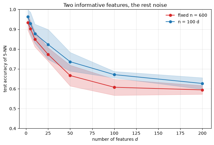
The first curve falls as the dimension grows although the informative structure never changes: the two useful features are still there, but they are buried among noise features, and the distances that k-NN trusts are dominated by the noise.
The second curve tests whether more data is the cure. It helps — every value is a little better than the corresponding point of the first curve — but it does not stop the decay: the accuracy still falls from about 0.96 at to about 0.63 at , with 33 times more data. More data buys density, and density was not the binding constraint here: the binding constraint is that nearly all coordinates are noise, so the distance concentration of the previous sections is a property of the distribution, not only of the sample size.
The practical consequence is the one ESL draws in §2.5: for high-dimensional data, k-NN must be preceded by something that removes or down-weights the uninformative directions — feature selection, PCA, or a learned metric. Adding points is useful, but it is not a substitute.
Summary¶
High-dimensional space is empty in the center: the volume of the ball is negligible compared with the cube, and almost all of the cube’s volume is in its corners.
A neighbourhood holding a fixed fraction of the points has edge length : in ten dimensions, 10% of the data needs 80% of the range of every coordinate.
Distances concentrate: , so neighbour rankings become noise and k-NN degrades — unless grows with .
Most of the volume of a ball is in a thin shell of fixed relative thickness, and Gaussian samples concentrate at radius with a thickness that does not grow with .
Uniform sampling in a ball needs the radius ; the easy way is a Gaussian direction times that radius. Rejection sampling dies exponentially.
Random vectors are nearly orthogonal, and pairwise distances are stable — the properties behind random projections.
References¶
Hastie et al. (2009), §2.5 (local methods in high dimensions, Figure 2.6) and §2.9 (model assessment).
Zaki & Meira (2020), chapter 6 (high-dimensional space, Figures 6.4–6.6).
Blum, Hopcroft and Kannan, Foundations of Data Science, chapter 2 (concentration of measure, random projections).
- Hastie, T., Tibshirani, R., & Friedman, J. (2009). The Elements of Statistical Learning: Data Mining, Inference, and Prediction (2nd ed.). Springer.
- Zaki, M. J., & Meira, W. (2020). Data Mining and Machine Learning: Fundamental Concepts and Algorithms (2nd ed.). Cambridge University Press. https://www.cambridge.org/9781108497367