k-Means: Objective, Lemmas and Lloyd’s Algorithm
Mahmood Amintoosi, Fall 2026
Computer Science Dept, Ferdowsi University of Mashhad
This page is the theory companion of Clustering: there scikit-learn is used to cluster digits and colours, and the algorithm is treated mostly as a black box. Here we ask what k-means actually minimizes, why the objective never increases, and how to write the algorithm from scratch.
Learning objectives. By the end you should be able to
write down the k-means objective and say what , and are in it;
prove the two identities behind the algorithm: that the centroid minimizes the sum of squared distances (Lemma 1, with its corollary), and that the same quantity can be computed from pairwise distances (Lemma 2);
prove that Lloyd’s algorithm terminates;
implement it safely — bounded iterations, empty clusters, a good initialization;
explain why the result is a local and not necessarily a global minimum, why that makes many restarts necessary, and what the result says when it is put against known labels.
Definition of Clustering¶
A clustering of a set of datapoints is a partition of the datapoints into disjoint subsets (or clusters) in such a way that datapoints in the same group are more similar (in some specific sense defined by the analyst) to each other than to those in other groups.
Representative-based Clustering¶
Given a dataset with points in a -dimensional space, , and given the number of desired clusters , the goal of representative-based clustering is to partition the dataset into groups or clusters, which is called a clustering and is denoted as .
For each cluster there exists a representative point that summarizes the cluster, a common choice being the mean (also called the centroid) of all points in the cluster, that is,
where is the number of points in cluster .
The k-means Objective¶
k-means is a representative-based clustering method: it partitions the datapoints into clusters by their similarity to the centroid of each cluster, and the partition it looks for is the one that minimizes the sum of squared distances between each datapoint and the centroid of its assigned cluster.
Lemma 1: Sum of Squared Distances to an Arbitrary Point¶
Let be a set of datapoints and let be their centroid. The sum of squared distances of the datapoints to any arbitrary point equals the sum of squared distances to the centroid plus the number of datapoints times the squared distance from to the centroid. That is,
Proof:
because the cross term vanishes: .
Corollary 1: The Centroid Minimizes the Sum of Squared Distances¶
For a fixed set of datapoints, the sum of squared distances to is minimized by , and is the unique minimizer. In other words, the centroid is the best representative of a cluster under the squared-error loss.
Proof:
In Lemma 1 the first two terms on the right do not depend on . The last term, , is non-negative and vanishes only when ; hence is the unique minimizer.
Lemma 2: Sum of Squared Distances Between All Pairs of Points¶
Let be a set of datapoints and let be their centroid. The sum of squared distances between all pairs of points equals times the sum of squared distances of the points to the centroid. That is,
Proof:
Lloyd’s Algorithm¶
The classical algorithm for k-means is Lloyd’s algorithm. It starts with initial centroids and alternates two steps until the assignment stops changing.
Initialize initial centroids (randomly, or with k-means++).
For each iteration, perform the following steps:
Assign each datapoint to the cluster whose centroid is nearest.
Update each centroid to the mean of all datapoints assigned to it.
Repeat step 2 until convergence.
Convergence of Lloyd’s Algorithm¶
Write the objective — the sum of squared errors (SSE) — as
and consider one full iteration, starting from the pair .
Assignment step. The centroids are held fixed and every point is moved to its nearest centroid. Each term can only decrease or stay the same, so the SSE does not increase.
Update step. The assignment is held fixed and each centroid is replaced by the mean of its cluster. By Corollary 1, for that fixed cluster the mean is the unique minimizer of ; the SSE does not increase again.
Termination. There are finitely many partitions of points into non-empty clusters, and the SSE is non-increasing, so it can change value only finitely many times. Once a full iteration leaves the assignment unchanged, the next iteration reproduces it exactly and the algorithm stops.
Two caveats matter in practice.
The argument proves convergence to a local minimum — a partition in which no single point can be reassigned so as to improve the objective — not to the global one. The result depends on the initial centroids and on how ties are broken.
The sequence is only non-increasing. If two centroids are exactly tied for a point, the assignment can oscillate between two equally good partitions; implementations therefore stop on a small tolerance or after a fixed number of iterations instead of testing exact equality of the centroids.
Implementing k-Means from Scratch¶
The class below is Lloyd’s algorithm, written so that the two failure modes of the naive
version are handled. The iteration is bounded by max_iter and stops on a tolerance rather
than on exact equality of the centroids, and an empty cluster keeps its previous centroid
instead of producing nan (the mean of an empty array is nan, and nan == nan is false,
so an exact-equality test would never terminate).
The initialisation is k-means++ by default: the first centroid is drawn uniformly from
the data, and each further centroid is drawn with probability proportional to its squared
distance to the closest centroid chosen so far. It is also the default of
sklearn.cluster.KMeans, and it is explained below.
import numpy as np
import matplotlib.pyplot as plt

SEED = 42


class KMeansClustering:
    """Lloyd's algorithm for k-means, with k-means++ initialisation."""

    def __init__(self, k, init="k-means++", seed=SEED):
        self.k = k
        self.init = init
        self.rng = np.random.default_rng(seed)
        self.centroids = None
        self.labels = None
        self.inertia = None

    def _initial_centroids(self, data):
        n = len(data)
        if self.init == "random":
            return data[self.rng.choice(n, size=self.k, replace=False)].copy()

        # k-means++: first centroid uniform, then D^2 sampling
        centroids = [data[self.rng.integers(n)]]
        for _ in range(1, self.k):
            d2 = ((data[:, None, :] - np.array(centroids)[None, :, :]) ** 2).sum(axis=2).min(axis=1)
            centroids.append(data[self.rng.choice(n, p=d2 / d2.sum())])
        return np.array(centroids, dtype=float)

    def fit(self, data, max_iter=300, tol=1e-9):
        data = np.asarray(data, dtype=float)
        self.centroids = self._initial_centroids(data)

        for iteration in range(max_iter):
            # 1. assignment step: each point to its nearest centroid
            distances = np.linalg.norm(data[:, None, :] - self.centroids[None, :, :], axis=2)
            self.labels = np.argmin(distances, axis=1)

            # 2. update step: each centroid to the mean of its cluster
            new_centroids = self.centroids.copy()
            for j in range(self.k):
                members = data[self.labels == j]
                if len(members) > 0:          # an empty cluster keeps its old centroid
                    new_centroids[j] = members.mean(axis=0)

            shift = np.max(np.abs(new_centroids - self.centroids))
            self.centroids = new_centroids
            if shift < tol:
                break

        self.n_iter_ = iteration + 1
        self.inertia = float(np.sum((data - self.centroids[self.labels]) ** 2))
        return self
The following script creates an instance of the KMeansClustering class, fits the model to the data, and plots the data with centroids and labels.
from sklearn.datasets import make_blobs

n_samples = 100
X, y = make_blobs(n_samples=n_samples, centers=3, n_features=2, random_state=SEED)

km = KMeansClustering(k=3).fit(X)

plt.figure(figsize=(6, 5))
plt.scatter(X[:, 0], X[:, 1], c=km.labels, cmap="viridis", s=30)
plt.scatter(km.centroids[:, 0], km.centroids[:, 1], marker="*", s=250, c="red",
            edgecolor="black", label="centroids")
plt.title(f"Lloyd's algorithm with k = 3 (SSE = {km.inertia:.1f}, {km.n_iter_} iterations)")
plt.legend(frameon=False)
plt.grid(alpha=0.3)
plt.show()

print("final centroids:")
print(np.round(km.centroids, 2))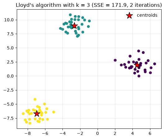
final centroids:
[[ 4.5   1.94]
 [-2.67  8.94]
 [-6.95 -6.68]]
Verifying Lemma 2 Numerically¶
Lemma 2 rewrites the SSE of a set of points — the quantity k-means minimizes — in terms of pairwise distances:
The left side sums over all pairs of points, the right side is times the sum of squared distances of the points to their centroid. The identity is useful whenever an algorithm can observe only pairwise distances and not the coordinates.
Note what Lemma 2 does not say: it is an identity, not an optimality statement. That the centroid minimizes the sum of squared distances is Corollary 1. Below we check that both sides of Lemma 2 give the same number for one cluster of the clustering above.
from scipy.spatial.distance import cdist


def lemma_2(points):
    """Compute both sides of Lemma 2 and report whether they agree."""
    n = len(points)
    centroid = points.mean(axis=0)
    right = n * np.sum((points - centroid) ** 2)
    left = np.sum(cdist(points, points) ** 2) / 2
    print(f"pairwise sum                         = {left:.6f}")
    print(f"n * sum of squared distances to mean = {right:.6f}")
    print(f"relative difference                  = {abs(left - right) / right:.2e}")
    return left, right


points = X[km.labels == 0]
print(f"cluster 0 contains {len(points)} points")
lemma_2(points)
cluster 0 contains 33 points
pairwise sum = 2042.432698
n * sum of squared distances to mean = 2042.432698
relative difference = 2.23e-16
(np.float64(2042.4326981762324), np.float64(2042.4326981762329))Cost¶
One iteration costs : the assignment step computes distances to each of centroids in dimensions, and the update step touches every point once. The number of iterations is small in practice (tens) but has no useful worst-case bound, which is why we cap it. The exact version can also be accelerated with a -d tree or with triangle-inequality bounds that skip most distance computations, and it can be replaced by the mini-batch approximation when is large; both are worked out in the appendix, together with the k-means++ initialisation that an earlier version of this page carried.
Example: Tumour Tissue Recovered by k-Means¶
The theory above says what k-means optimizes; it does not say whether the answer is worth anything on real data. The standard test is the human tumour microarray data of Hastie et al. (2009) (§14.3.8, pp. 512–514), used there to illustrate high-dimensional clustering:
the matrix is 6830 genes × 64 samples of expression measurements;
the objects to cluster are the samples, so sample is a point in , and two samples are close when their whole profiles agree, not when one gene agrees;
every sample also carries a pathology label — breast, CNS, colon, K562, leukemia, MCF7, melanoma, NSCLC, ovarian, prostate, renal, unknown — which is withheld during clustering and used only afterwards, to ask what each cluster turned out to contain.
The first lesson of the example is that is not in the data. Plotting the total within-cluster sum of squares against gives no clear kink (Figure 14.8 of the book), so is chosen as a deliberate coarsening: eleven tissue types squeezed into three boxes.
Running k-means with and then counting which labels landed where gives Table 14.2 of the book — the form in which a clustering should be reported whenever labels exist, because it shows both the clean groups and the mistakes:
| Cluster | Breast | CNS | Colon | K562 | Leukemia | MCF7 | Melanoma | NSCLC | Ovarian | Prostate | Renal | Unknown |
|---|---|---|---|---|---|---|---|---|---|---|---|---|
| 1 | 3 | 5 | 0 | 0 | 0 | 0 | 1 | 7 | 6 | 2 | 9 | 1 |
| 2 | 2 | 0 | 0 | 2 | 6 | 2 | 7 | 2 | 0 | 0 | 0 | 0 |
| 3 | 2 | 0 | 7 | 0 | 0 | 0 | 0 | 0 | 0 | 0 | 0 | 0 |
Read it by rows. Cluster 3 is essentially the colon cancers: all seven of them, plus two breast samples, and no colon sample appears anywhere else. Cluster 2 collects the blood and skin tumours — the six leukemias with the K562 and MCF7 lines, the melanomas, and two NSCLC samples. Cluster 1 is the remainder (CNS, ovarian, renal, prostate, most NSCLC), the largest and least pure group, which is what one expects when eleven types are forced into three clusters. The algorithm never saw a single label.
What the example is worth, and what it does not settle¶
The two breast samples in cluster 2 turned out to be melanomas that had metastasized; the clustering was right against the label. It is worth being precise about what that means: the algorithm produced a suspicion — these profiles look like that group, not like the group their labels claim — and a pathologist confirmed it afterwards. Without the re-examination the honest conclusion would have been “two samples are inconsistent with their labels, for reasons unknown”. Unsupervised learning can be right against its labels, but only a follow-up turns that into knowledge.
Two limits of the method are visible in the same table:
no order inside a cluster: cluster 1 can only be listed alphabetically, which says nothing about which of its members are most alike;
no nesting across : the solution need not refine the solution, so a table built for one cannot be extended when the number of groups is revised.
Both are cured by the same change of report: a dendrogram orders the samples along a line and gives a nested family of partitions, which is why the book calls hierarchical clustering preferable for this application. Everything else here is small- caution: with one atypical sample moves a centroid and changes the table visibly, the choice of genes and the preprocessing move every distance, and a single run with a random start proves nothing — the guard is many restarts, or the improved initialisation treated in the appendix.
Summary¶
k-means minimizes the SSE over partitions into non-empty clusters.
Lemma 1 decomposes the sum of squared distances to an arbitrary point ; its corollary identifies the centroid as the unique minimizer, which is what justifies the update step.
Lemma 2 rewrites the SSE through pairwise distances. It is an identity, not an optimality statement.
Lloyd’s algorithm alternates assignment and update, so the SSE never increases; a non-increasing sequence over a finite set of partitions must stop, at a local minimum.
The result depends on the initialization, so implementations restart the whole procedure a few times and keep the run with the smallest SSE; k-means++ and the experiment behind it are in the appendix.
On the tumour microarray example, k-means recovers tissue of origin without seeing a single label, and the contingency table — not the clusters themselves — is the result.
Choosing is a separate problem, treated in Clustering Validation.
Optional materials related to k-means¶
Where the rest of this material lives¶
Two appendix pages carry what did not fit here:
Appendix: Further Clustering Measures and k-Means Variants — NMI and its missing chance correction, the gap statistic that turns the elbow into a decision, the assignment problem behind the maximum-matching score, the k-means++ initialisation with its 100-run experiment, and mini-batch k-means with a timing comparison against the exact algorithm.
Appendix: From the k-Means Objective to Lloyd’s Algorithm — the same objective opened with calculus: differentiating it with respect to a centroid gives the centroid step, the assignment step is linear in the one-hot assignment and attains its minimum at a vertex, alternating the two steps is Lloyd’s algorithm, the matrix form previews the normal equations of regression, and a procedural Iris implementation checks every formula numerically.
- Hastie, T., Tibshirani, R., & Friedman, J. (2009). The Elements of Statistical Learning: Data Mining, Inference, and Prediction (2nd ed.). Springer.