Linear Regression, Part 2¶

Computer Science Dept, Ferdowsi University of Mashhad

Just as naive Bayes (discussed in Naive Bayes Classification) is a good starting point for classification tasks, linear regression models are a good starting point for regression tasks. Such models are popular because they can be fit quickly and are straightforward to interpret. You are already familiar with the simplest form of linear regression model (i.e., fitting a straight line to two-dimensional data), but such models can be extended to model more complicated data behavior.

Linear Model¶

Suppose that the true model is denoted by $y = b + m x + \epsilon$ and the estimated model denoted by $\hat{y}$ (Eq. 23.2 of Zaki book Zaki & Meira (2020)):

\begin{aligned} \\ \hat{y} &= \beta_0 + \beta_1 x \\ &= \beta_0 x_0+ \beta_1 x_1 \quad \ \textrm{(ESL Notation)}\\ &= \theta_0 x_0+ \theta_1 x_1 \quad \ \ \textrm{(Ng Notation)}\\ &= w_0 x_0+ w_1 x_1 \quad\textrm{(Zaki Notation)}\\ \\ &\textrm{where:}\\ &x_0 = 1 \end{aligned}

(1)

If we have:

\mathbf{x} = \begin{bmatrix} x_0\\x_1 \end{bmatrix}, \mathbf{w} = \begin{bmatrix} w_0\\w_1 \end{bmatrix}

(2)

then $\hat{y}$ can be considered as dot product of two vectors:

\begin{aligned} \hat{y} = w_0 x_0+ w_1 x_1 = \mathbf{w}^T\mathbf{x} \end{aligned}

(3)

If $i^{th}$ instance is shown by $\mathbf{x}_i$

\mathbf{x}_i = \begin{bmatrix} x_{i,0}\\x_{i,1} \end{bmatrix},

(4)

then:

\begin{aligned} \hat{y}_i = w_0 x_{i,0}+ w_1 x_{i,1} \end{aligned}

(5)

Sum of Squared Error (SSE):

\begin{aligned} \textrm{SSE} &= \sum_{i=1}^n{error_i}^2 \\ &= \sum_{i=1}^n{(\hat{y_i} - y_i)}^2 \\ &= \sum_{i=1}^n{(w_0 x_{i,0} + w_1 x_{i,1} - y_i)}^2\\ &= \sum_{i=1}^n{(\mathbf{w}^T\mathbf{x}_{i} - y_i)}^2 = \sum_{i=1}^n{(\mathbf{x}_{i}^T\mathbf{w} - y_i)}^2\\ &= ||X\mathbf{w} - \mathbf{y}||_2^2 = (X\mathbf{w} - \mathbf{y})^T(X\mathbf{w} - \mathbf{y}) \end{aligned}

(6)

where:

X = \begin{bmatrix} \mathbf{x_1}^T \\ \mathbf{x_2}^T \\ \vdots \\ \mathbf{x_n}^T \end{bmatrix}, \mathbf{y} = \begin{bmatrix} y_1 \\ y_2 \\ \vdots \\ y_n \end{bmatrix}

(7)

Data Generation¶

Synthetic Data Generation¶

true_w0 = 1  # b in mx+b
true_w1 = 2  # m in mx+b
N = 100

# Data Generation
np.random.seed(42)
x = np.random.rand(N, 1)

epsilon = 0.1 * np.random.randn(N, 1)
y = true_w0 + true_w1 * x + epsilon

# Add a column of 1s to x

# ones = np.ones((N, 1))
# X = np.concatenate([ones, x],axis=1)
X = np.insert(x, 0, 1, axis=1)
print(x.shape, X.shape)
print(x[:3])
print(y[:3])

(100, 1) (100, 2)
[[0.37454012]
 [0.95071431]
 [0.73199394]]
[[1.75778494]
 [2.87152788]
 [2.47316396]]

figure0(x, y)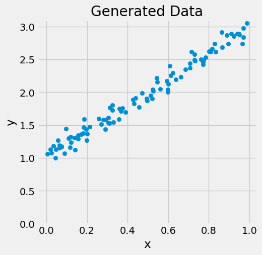

Normal Equations¶

The Normal Equations provide a closed-form solution for finding the optimal parameters (coefficients) that minimize the cost function (usually the mean squared error) in linear regression.

The Normal Equations are derived by setting the partial derivatives of the cost function with respect to each coefficient to zero.
The Closed Form Solution refers to finding the optimal parameters directly using a mathematical formula, rather than an iterative optimization process.

We have to minimize: $||X\mathbf{w} - \mathbf{y}||_2^2$ wrt $\mathbf{w}$ , which is equal to the famous form $min_{x}||Ax - b||_2^2$ . Temporary we use $\beta$ , instead of $\mathbf{w}$ and ignore the bold faces of letters; hence we have to minimize $||X\beta-y||_2^2$

\begin{aligned} SSE&=||X\beta-y||_2^2 = (X\beta-y)^T(X\beta-y)\\ &=((X\beta)^T-y^T)(X\beta-y) =(\beta^TX^T-y^T)(X\beta-y) \\ &=\beta^TX^T X\beta - \beta^T X^Ty -y^TX\beta + y^Ty\\ &=\beta^T M\beta - (X\beta)^Ty -y^TX\beta + y^Ty \qquad {(M=X^T X)}\\ &=\beta^T M\beta - 2y^TX\beta + y^Ty \qquad\qquad{(A^TB=B^TA)}\\ &=\beta^T M\beta - 2z^T\beta + y^Ty \qquad\qquad{(z^T=y^TX, z=X^Ty)} \end{aligned}

(8)

We Know that (See Matrix Calculus in Wikipedia):

\frac{\partial y^Tx}{\partial x}=\frac{\partial x^Ty}{\partial x}=y

(9)

\frac{\partial Mx}{\partial x}=M

(10)

and if $M$ be a symmetric matrix:

\frac{\partial x^TMx}{\partial x}=2Mx

(11)

Hence:

\begin{aligned} \frac{\partial SSE}{\partial \beta} &= \frac{\partial (\beta^T M\beta - 2z^T\beta + y^Ty)}{\partial \beta} \\ &= 2M\beta-2z = 2X^TX\beta-2X^T y \end{aligned}

(12)

Set the derivative equal to zero:

\begin{aligned} &\frac{\partial SSE}{\partial \beta}=0 \\ \Rightarrow & 2 X^TX\beta - 2X^T y = 0\\ \Rightarrow & X^TX\beta = X^Ty \\ \Rightarrow & \beta = (X^TX)^{-1}X^Ty \\ \end{aligned}

(13)

and with our previous notation: $\mathbf{w} = (X^TX)^{-1}X^T\mathbf{y}$

w = np.linalg.inv(X.T @ X) @ X.T @ y
w

array([[1.02150962],
       [1.95402268]])

Using Scikit-learn¶

from sklearn.linear_model import LinearRegression

linreg = LinearRegression()
linreg.fit(x, y)
print(linreg.intercept_, linreg.coef_)

[1.02150962] [[1.95402268]]

If we have augmented data matrix $X \in \mathbb{R}^{n\times (d+1)}$ , we have to set fit_intercept=False. In eq. (23.20) of Zaki this is denoted by $\tilde{D}$ .

linreg = LinearRegression(fit_intercept=False)
linreg.fit(X, y)
print(linreg.coef_)

[[1.02150962 1.95402268]]

Bivariate Regression¶

In bivariate regression, we have two variables: one is the predictor variable (also known as the feature), and the other is the response variable (also known as the target).

Predictor Variable (Feature):
- The predictor variable (often denoted as x) is the input variable that we use to predict or explain the variation in the response variable.
- In machine learning, this is equivalent to a feature. Features represent the characteristics or attributes of the data points.
- For example, in a housing price prediction model, features could include square footage, number of bedrooms, location, etc.
Response Variable (Target):
- The response variable (often denoted as y) is the output variable that we are trying to predict or understand based on the predictor variable.
- In machine learning, this is equivalent to the target. The target represents the value we want to predict.
- For the housing price prediction model, the target would be the actual sale price of a house.

So, in summary, bivariate regression involves analyzing the relationship between two variables: one (the feature) is used to predict or explain the behavior of the other (the target). These terms are commonly used in both statistics and machine learning.

For further information about Multivariate Multiple Regression, see this blog post of Faradars.

Gradient Descent¶

In this section we are going to introduce the basic concepts underlying gradient descent. Some materials are borrowed from D2L.

One-Dimensional Gradient Descent¶

Gradient descent in one dimension is an excellent example to explain why the gradient descent algorithm may reduce the value of the objective function. Consider some continuously differentiable real-valued function $f: \mathbb{R} \rightarrow \mathbb{R}$ . Using a Taylor expansion we obtain

f(x + h) = f(x) + h f'(x) + \mathcal{O}(h^2).

(14)

That is, in first-order approximation $f(x+h)$ is given by the function value $f(x)$ and the first derivative $f'(x)$ at $x$ . It is not unreasonable to assume that for small $h$ moving in the direction of the negative gradient will decrease $f$ . To keep things simple we pick a fixed step size $\eta > 0$ and choose $h = -\eta f'(x)$ . Plugging this into the Taylor expansion above we get

f(x - \eta f'(x)) = f(x) - \eta f'^2(x) + \mathcal{O}(\eta^2 f'^2(x)).

(15)

If the derivative $f'(x) \neq 0$ does not vanish we make progress since $\eta f'^2(x)>0$ . Moreover, we can always choose $\eta$ small enough for the higher-order terms to become irrelevant. Hence we arrive at

f(x - \eta f'(x)) \lessapprox f(x).

(16)

This means that, if we use

x \leftarrow x - \eta f'(x)

(17)

to iterate $x$ , the value of function $f(x)$ might decline. Therefore, in gradient descent we first choose an initial value $x$ and a constant $\eta > 0$ and then use them to continuously iterate $x$ until the stop condition is reached, for example, when the magnitude of the gradient $|f'(x)|$ is small enough or the number of iterations has reached a certain value.

Gradient Descent on $f(x)=x^2$ ¶

For simplicity we choose the objective function $f(x)=x^2$ to illustrate how to implement gradient descent. Although we know that $x=0$ is the solution to minimize $f(x)$ , we still use this simple function to observe how $x$ changes.

# Defining a simple quadratic function and its derivative
f = lambda x: x**2
f_prime = lambda x: 2 * x

# Generating values
x = np.linspace(-10, 10, 400)
y = f(x)

# Gradient descent settings
learning_rate = 0.1
x_start = 9.0  # Starting point
steps = [x_start]
n_iterations = 15

# Gradient Descent Iteration
for _ in range(n_iterations):
    print(
        "x = {:4.2f}, f'(x) = {:5.2f}, -lr*f'(x)={:5.2f}".format(
            x_start, f_prime(x_start), -learning_rate * f_prime(x_start)
        )
    )
    x_start = x_start - learning_rate * f_prime(x_start)
    steps.append(x_start)

# Plotting the function
plt.figure(figsize=(8, 5))
plt.plot(x, y, lw=2, color="blue", label="f(x) = x²")

# Plotting the steps
plt.scatter(steps, f(np.array(steps)), color="red", s=100, label="Steps")
plt.plot(steps, f(np.array(steps)), color="red", linestyle="--", lw=1.5)

# Annotations and labels
plt.title("Gradient Descent on f(x) = x²")
plt.xlabel("x")
plt.ylabel("f(x)")
plt.legend()
plt.grid(True)
plt.show()

x = 9.00, f'(x) = 18.00, -lr*f'(x)=-1.80
x = 7.20, f'(x) = 14.40, -lr*f'(x)=-1.44
x = 5.76, f'(x) = 11.52, -lr*f'(x)=-1.15
x = 4.61, f'(x) =  9.22, -lr*f'(x)=-0.92
x = 3.69, f'(x) =  7.37, -lr*f'(x)=-0.74
x = 2.95, f'(x) =  5.90, -lr*f'(x)=-0.59
x = 2.36, f'(x) =  4.72, -lr*f'(x)=-0.47
x = 1.89, f'(x) =  3.77, -lr*f'(x)=-0.38
x = 1.51, f'(x) =  3.02, -lr*f'(x)=-0.30
x = 1.21, f'(x) =  2.42, -lr*f'(x)=-0.24
x = 0.97, f'(x) =  1.93, -lr*f'(x)=-0.19
x = 0.77, f'(x) =  1.55, -lr*f'(x)=-0.15
x = 0.62, f'(x) =  1.24, -lr*f'(x)=-0.12
x = 0.49, f'(x) =  0.99, -lr*f'(x)=-0.10
x = 0.40, f'(x) =  0.79, -lr*f'(x)=-0.08

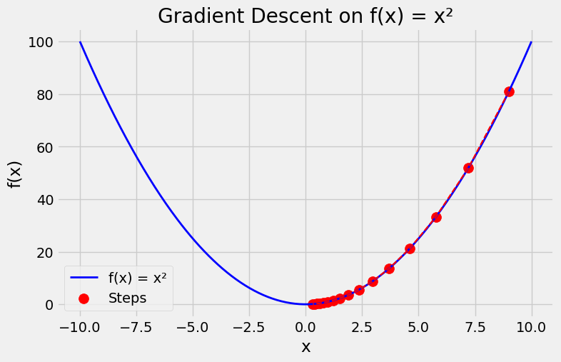
And another function see $f(x)=3\sin(x)+(0.1x-3)^2$ where is solved in ADS course using PSO.

# Defining a simple quadratic function and its derivative
f = lambda x: 3 * np.sin(x) + (0.1 * x - 3) ** 2
f_prime = lambda x: 3 * np.cos(x) + 0.2 * (0.1 * x - 3)

# Generating values
x = np.linspace(0, 60, 400)
y = f(x)

# Gradient descent settings
learning_rate = 0.1
x_start = 20  # Starting point
steps = [x_start]
n_iterations = 15

# Gradient Descent Iteration
for _ in range(n_iterations):
    x_start = x_start - learning_rate * f_prime(x_start)
    steps.append(x_start)

# Plotting the function
plt.figure(figsize=(8, 6))
plt.plot(x, y, lw=2, color="blue", label="f(x) = 3sin(x)+(0.1x-3)²")

# Plotting the steps
plt.scatter(steps, f(np.array(steps)), color="red", s=100, label="Steps")
plt.plot(steps, f(np.array(steps)), color="red", linestyle="--", lw=1.5)

# Annotations and labels
plt.title("Gradient Descent on f(x) = 3sin(x)+(0.1x-3)²")
plt.xlabel("x")
plt.ylabel("f(x)")
plt.legend()
plt.grid(True)
plt.show()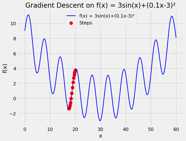

Using Gradient Descent for Regression in Machine Learning¶

Here we use training data for estimation of the model parameters and report the error on test data

# Reproduce our data
true_w0 = 1  # b in mx+b
true_w1 = 2  # m in mx+b
N = 100

# Data Generation
np.random.seed(42)
x = np.random.rand(N, 1)

epsilon = 0.1 * np.random.randn(N, 1)
y = true_w0 + true_w1 * x + epsilon
X = np.insert(x, 0, 1, axis=1)

Train-Test Split¶

x_train, x_test, y_train, y_test = train_test_split(X, y, test_size=0.2)

x_train.shape, y_train.shape

((80, 2), (80, 1))

figure1(x_train, y_train, x_test, y_test)

(<Figure size 1200x600 with 2 Axes>,
 array([<Axes: title={'center': 'Generated Data - Train'}, xlabel='x', ylabel='y'>,
        <Axes: title={'center': 'Generated Data - Test'}, xlabel='x', ylabel='y'>],
       dtype=object))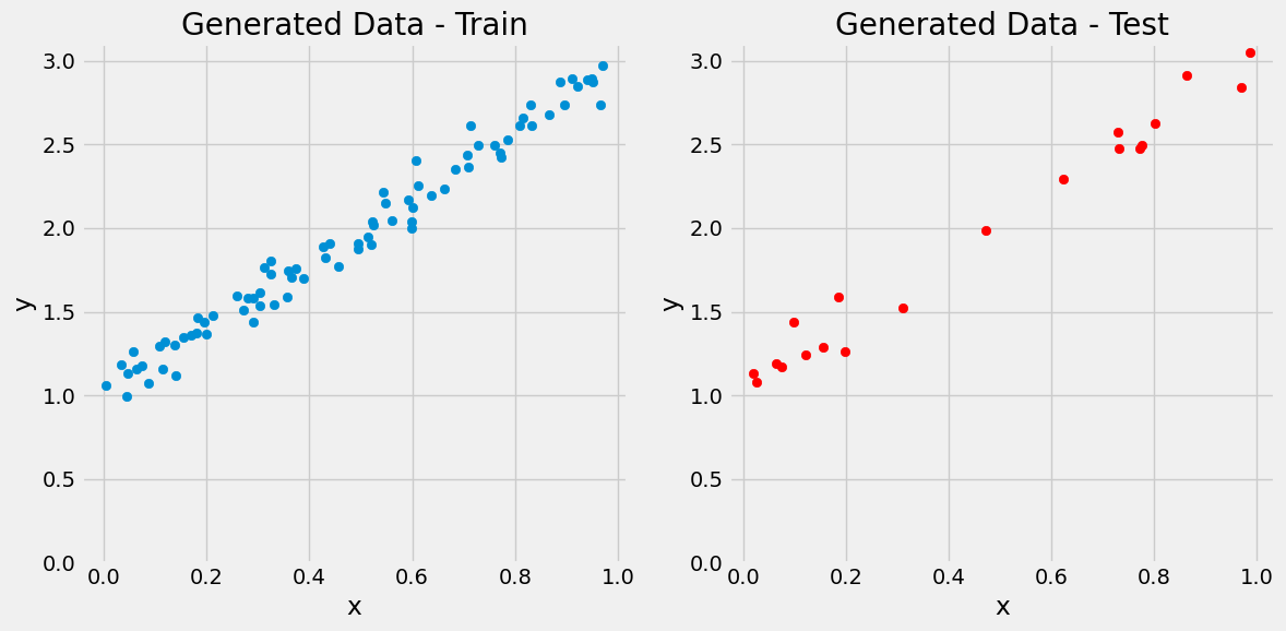

Step 0: Random Initialization¶

# Step 0 - Initializes parameters "b" and "w" randomly
np.random.seed(42)
w = np.random.randn(2, 1)
print(w)

[[ 0.49671415]
 [-0.1382643 ]]

Step 1: Compute Model’s Predictions¶

# Step 1 - Computes our model's predicted output - forward pass
# y_hat = b + m * x_train
y_hat = w[0] + w[1] * x_train[:, 1]
y_hat[:3]

array([0.39881299, 0.41404593, 0.36925186])

y_hat = x_train @ w
y_hat[:3]

array([[0.39881299],
       [0.41404593],
       [0.36925186]])

figure2(x_train, y_train, w[0], w[1])

(<Figure size 600x600 with 1 Axes>, <Axes: xlabel='x', ylabel='y'>)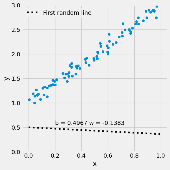

Step 2: Compute the Loss¶

$$

\begin{aligned} error_i &= \hat{y_i} - y_i\ where:\ y &= true_w_0 + true_w_1 x_1 + \epsilon\ &\hat{y}= w_0 x_0+ w_1 x_1 \end{aligned} $$

print(y_train[0], y_hat[0])
figure3(x_train, y_train, w[0], w[1])

[2.36596945] [0.39881299]

(<Figure size 600x600 with 1 Axes>, <Axes: xlabel='x', ylabel='y'>)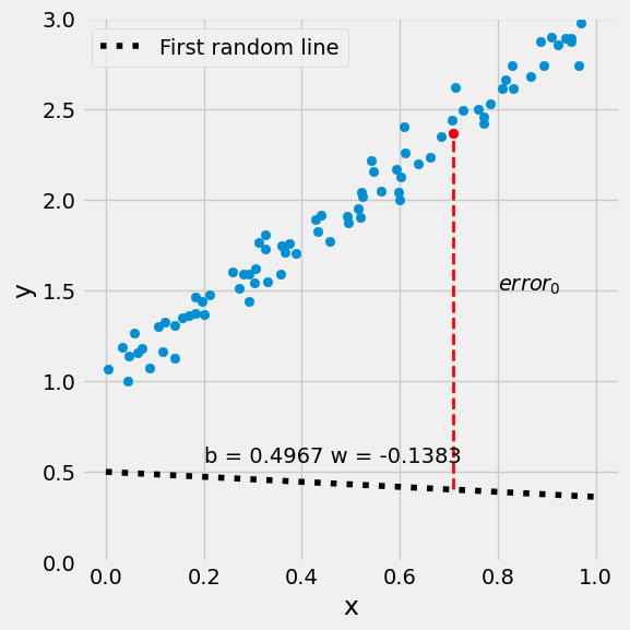

$$

\begin{aligned} MSE &= \frac{1}{n} \sum_{i=1}^n{error_i}^2 \ &= \frac{1}{n} \sum_{i=1}^n{(\hat{y_i} - y_i)}^2 \ &= \frac{1}{n} \sum_{i=1}^n{(w_0 x_{i,0} + w_1 x_{i,1} - y_i)}^2 \end{aligned} $$

# Step 2 - Computing the loss
# We are using ALL data points, so this is BATCH gradient
# descent. How wrong is our model? That's the error!
error = y_hat - y_train
print(error.shape)
# It is a regression, so it computes mean squared error (MSE)
loss = (error**2).mean()
print(loss)

(80, 1)
2.6401126993616817

Loss Surface¶

w0s, w1s, all_losses = mesh_losses(true_w0, true_w1, x_train, y_train)

figure4(x_train, y_train, w[0], w[1], w0s, w1s, all_losses)

(<Figure size 1200x600 with 2 Axes>,
 (<Axes3D: title={'center': 'Loss Surface'}, xlabel='b', ylabel='w'>,
  <Axes: title={'center': 'Loss Surface'}, xlabel='b', ylabel='w'>))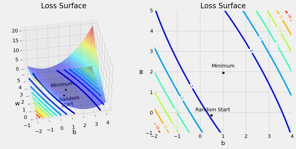

Step 3: Compute the Gradients¶

\begin{aligned} \frac{\partial{MSE}}{\partial{w_j}} &= \frac{\partial{}}{\partial{w_j}}\frac{1}{n} \big(\sum_{i=1}^n{error_i}^2\big) =\frac{1}{n} \sum_{i=1}^n{\frac{\partial{error_i^2}}{\partial{w_j}}} \\ &= \frac{1}{n} \sum_{i=1}^n{\frac{\partial{{(\hat{y_i} - y_i)}^2}}{\partial{w_j}}} \\ &= \frac{1}{n} \sum_{i=1}^n{2\frac{\partial{(\hat{y_i} - y_i)}}{\partial{w_j}} (\hat{y_i} - y_i)}\\ &= \frac{1}{n} \sum_{i=1}^n{2\frac{\partial{(\hat{y_i} - y_i)}}{\partial{\hat{y_i}}} \cdot \frac{\partial{\hat{y_i}}}{\partial{w_j}} (\hat{y_i} - y_i)} \\ &= 2 \frac{1}{n} \sum_{i=1}^n{x_{i,j} (\hat{y_i} - y_i)}= 2 \frac{1}{n} \sum_{i=1}^n{x_{i,j} error_i} \end{aligned}

(18)

# Step 3 - Computes gradients for both "b" and "w" parameters
w0_grad = 2 * error.mean()
# w1_grad = 2 * (x_train[:,1] * error).mean() # Wrong!
w1_grad = 2 * (np.delete(x_train, 0, axis=1) * error).mean()
print(w0_grad, w1_grad)

-3.0224384959608583 -1.7706733515907813

(x_train * error).shape

(80, 2)

Vectorized form

# w_grad = 2 * (x_train * error).mean() # Wrong
w_grad = 2 * (x_train * error).mean(axis=0)
print(w_grad.shape, w_grad)
w_grad = np.reshape(w_grad, (2, 1))
print(w_grad.shape, w_grad)

(2,) [-3.0224385  -1.77067335]
(2, 1) [[-3.0224385 ]
 [-1.77067335]]

Backpropagation¶

Step 4: Update the Parameters¶

$$

\begin{aligned} & b = b - \eta \frac{\partial{MSE}}{\partial{b}} \ & w = w - \eta \frac{\partial{MSE}}{\partial{w}} \end{aligned} $$

print(w.shape, w_grad.shape)

(2, 1) (2, 1)

# Sets learning rate - this is "eta" ~ the "n" like Greek letter
lr = 0.1
print(w[0], w[1])

# Step 4 - Updates parameters using gradients and the
# learning rate
# w[0] = w[0] - lr * w0_grad
# w[1] = w[1] - lr * w1_grad
w = w - lr * w_grad

print(w)
print(w[0])

[0.49671415] [-0.1382643]
[[0.798958  ]
 [0.03880303]]
[0.798958]

figure9(x_train, y_train, w[0], w[1])

(<Figure size 600x600 with 1 Axes>, <Axes: xlabel='x', ylabel='y'>)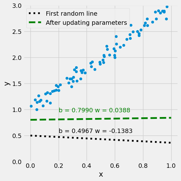

Step 5: Repeat the above updating!¶

# Initializes parameters "b" and "w" randomly
np.random.seed(42)
w = np.random.randn(2, 1)
lr = 0.3
num_epochs = 50
Losses = np.empty(num_epochs)
for epoch in range(num_epochs):
    y_hat = x_train @ w
    error = y_hat - y_train
    loss = (error**2).mean()
    Losses[epoch] = loss
    w_grad = 2 * (x_train * error).mean(axis=0)
    w_grad = np.reshape(w_grad, (2, 1))
    w = w - lr * w_grad

w

array([[1.11648206],
       [1.75056848]])

figure9(x_train, y_train, w[0], w[1])

(<Figure size 600x600 with 1 Axes>, <Axes: xlabel='x', ylabel='y'>)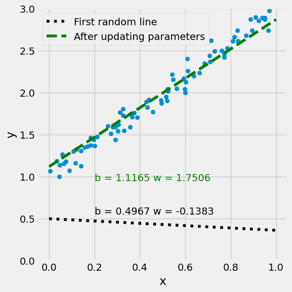

plt.plot(Losses)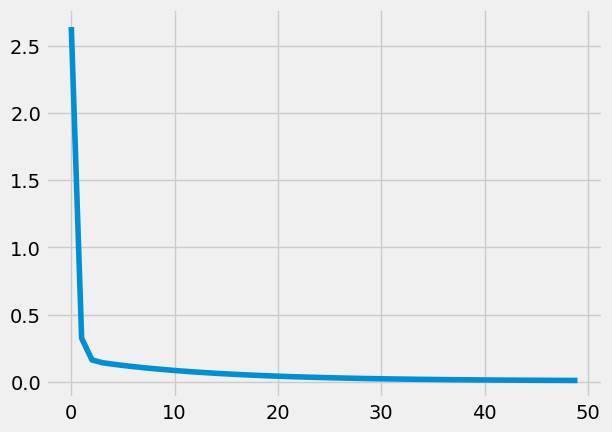

Using PyTorch auto grad¶

PyTorch is a Python-based tool for scientific computing that provides several main features:
- torch.Tensor, an n-dimensional array similar to that of numpy, but which can run on GPUs
- Computational graphs for building neural networks
- Automatic differentiation for training neural networks (more on this next lecture)
You can install PyTorch from: https://pytorch.org/

import torch
from torch import autograd

# Initializes parameters "b" and "w" randomly
np.random.seed(42)
b = np.random.randn(1)
w = np.random.randn(1)

b = torch.tensor(b, requires_grad=True)
w = torch.tensor(w, requires_grad=True)
xTrain = torch.tensor(x_train)  # xTrain is a pyTorch Tensor
yTrain = torch.tensor(y_train)  # yTrain is a pyTorch Tensor

Backward¶

Differntiationg using backward function

https://pytorch.org/tutorials/beginner/pytorch_with_examples.html

np.random.seed(42)
w = np.random.randn(2, 1)

w = torch.tensor(w, requires_grad=True)
xTrain = torch.tensor(x_train)  # xTrain is a pyTorch Tensor
yTrain = torch.tensor(y_train)  # yTrain is a pyTorch Tensor

lr = 0.3
num_epochs = 50
for epoch in range(num_epochs):
    y_hat = xTrain @ w
    error = y_hat - yTrain
    loss = (error**2).mean(axis=0)
    # removed the manual derivative computation and use autograd instead
    loss.backward()
    with torch.no_grad():
        w -= lr * w.grad
        # Manually zero the gradients after updating weights
        w.grad = None

w

tensor([[1.1165],
        [1.7506]], dtype=torch.float64, requires_grad=True)

https://pytorch.org/tutorials/beginner/pytorch_with_examples.html

PyTorch: Defining new autograd functions
PyTorch: nn module
PyTorch: optim
PyTorch: Custom nn Modules

Using PyTorch library¶

import torch
import torch.nn as nn

# x_train.dtype is float64, so cast both inputs to float32
xTrain = torch.tensor(x_train, dtype=torch.float32)
yTrain = torch.tensor(y_train, dtype=torch.float32)

# the same simple model as before: one input, one output, with bias
# now that the data has two columns we either use the second column only
# or define the model without a bias
model = nn.Linear(2, 1, bias=False)

learning_rate = 0.3
f = nn.MSELoss()
optimizer = torch.optim.SGD(model.parameters(), lr=learning_rate)

num_epochs = 50
for epoch in range(num_epochs):
    y_hat = model(xTrain)
    loss = f(y_hat, yTrain)
    loss.backward()  # backward propagation: calculate gradients
    optimizer.step()  # update the weights
    optimizer.zero_grad()  # clear out the gradients from the last step loss.backward()

print(model)
print(model.bias)
print(model.weight)
print(model.weight[0])
print(model.weight[0][0])
print(model.weight[0][0].item())
print(model.weight[0].detach().numpy()[0])

Linear(in_features=2, out_features=1, bias=False)
None
Parameter containing:
tensor([[1.0971, 1.7887]], requires_grad=True)
tensor([1.0971, 1.7887], grad_fn=<SelectBackward0>)
tensor(1.0971, grad_fn=<SelectBackward0>)
1.0971075296401978
1.0971075

w = model.weight[0].detach().numpy()
w = np.reshape(w, (2, 1))
figure9(x_train, y_train, w[0], w[1])

(<Figure size 600x600 with 1 Axes>, <Axes: xlabel='x', ylabel='y'>)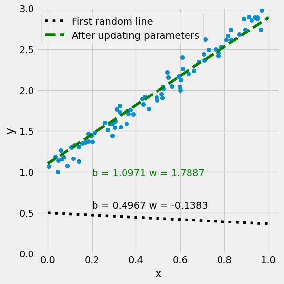

Further Reading:

Linear Regression, Part 2

Linear Regression, Part 2¶

Linear Model¶

Data Generation¶

Synthetic Data Generation¶

Normal Equations¶

Using Scikit-learn¶

Bivariate Regression¶

Gradient Descent¶

One-Dimensional Gradient Descent¶

Gradient Descent on f(x)=x2f(x)=x^2f(x)=x2¶

Using Gradient Descent for Regression in Machine Learning¶

Train-Test Split¶

Step 0: Random Initialization¶

Step 1: Compute Model’s Predictions¶

Step 2: Compute the Loss¶

Loss Surface¶

Step 3: Compute the Gradients¶

Backpropagation¶

Step 4: Update the Parameters¶

Step 5: Repeat the above updating!¶

Using PyTorch auto grad¶

Backward¶

Using PyTorch library¶

Gradient Descent on $f(x)=x^2$ ¶