Neural Networks for Classification¶

Mahmood Amintoosi, Fall 2026

Computer Science Dept, Ferdowsi University of Mashhad

I should mention that the original material was from Tomas Beuzen’s course.

Lecture Learning Objectives¶

Logistic Regression
Classification using Neural Networks

Imports¶

# Auto-setup when running on Google Colab
import os
if 'google.colab' in str(get_ipython()) and not os.path.exists('/content/neural-networks'):
    !git clone -q https://github.com/fum-cs/neural-networks.git /content/neural-networks
    !pip --quiet install -r /content/neural-networks/requirements_colab.txt
    %cd neural-networks/notebooks

import warnings
warnings.filterwarnings('ignore')
import sys
import numpy as np
import pandas as pd
import torch
from torchsummary import summary
from torch import nn, optim
from torch.utils.data import DataLoader, TensorDataset
from sklearn.datasets import make_regression, make_circles, make_blobs
from sklearn.preprocessing import StandardScaler
from sklearn.linear_model import LinearRegression, LogisticRegression
from scipy.optimize import minimize
from utils.plotting import *
import plotly.io as pio
pio.renderers.default = 'notebook'

Logistic Regression¶

In this section I’m going to demo optimizing a Logistic Regression problem to drive home some of the points we learned in the previous lectures
I’m going to sample 70 “legendary” (which are typically super-powered) and “non-legendary” pokemon from our dataset

df = pd.read_csv("data/pokemon.csv", index_col=0, usecols=['name', 'defense', 'legendary']).reset_index()
leg_ind = df["legendary"] == 1
df[leg_ind].head(5), df[~leg_ind].head(5)

(         name  defense  legendary
 143  Articuno      100          1
 144    Zapdos       85          1
 145   Moltres       90          1
 149    Mewtwo       70          1
 150       Mew      100          1,
          name  defense  legendary
 0   Bulbasaur       49          0
 1     Ivysaur       63          0
 2    Venusaur      123          0
 3  Charmander       43          0
 4  Charmeleon       58          0)

df = pd.concat(
    (df[~leg_ind].sample(sum(leg_ind), random_state=123), df[leg_ind]),
    ignore_index=True,
).sort_values(by='defense',ascending=False)

x = StandardScaler().fit_transform(df[['defense']]).flatten()  # we saw before the standardizing is a good idea for optimization
y = df['legendary'].to_numpy()
plot_logistic(x, y)

We’ll be using the “trick of ones” to help us implement these computations efficiently
For example, if we have a simple linear regression model with an intercept and a slope:

\hat{y} = \boldsymbol{w^T}\boldsymbol{x} = w_0\times{}1 + w_1\times{}x

(1)

Let’s represent that in matrix form:

\begin{bmatrix} y_1 \\ y_2 \\ \vdots \\ y_n \end{bmatrix}=\begin{bmatrix} 1 & x_1 \\ 1 & x_2 \\ \vdots & \vdots \\ 1 & x_n \end{bmatrix} \begin{bmatrix} w_0 \\ w_1 \end{bmatrix}

(2)

Now we can calculate $\mathbf{y}$ using matrix multiplication and the “matmul” Python operator:

w = np.array([2, 3])
X = np.array([[1, 5], [1, 3], [1, 4]])
X @ w

array([17, 11, 14])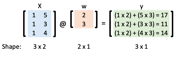

We’re going to create a logistic regression model to classify a Pokemon as “legendary” or not
In logistic regression we map our linear model to a probability:

z=\boldsymbol{w^T}\boldsymbol{x}

(3)

P(y = 1) = \frac{1}{(1+\exp(-z))}

(4)

For classification purposes, we typically then assign this probability to a discrete class (0 or 1) based on a threshold (0.5 by default):

y=\left\{ \begin{array}{ll} 0, & P(y = 1)\le0.5 \\ 1, & P(y = 1)>0.5 \\ \end{array} \right.

(5)

Let’s code that up:

def sigmoid(x, w, output="soft", threshold=0.5):
    p = 1 / (1 + np.exp(-x @ w))
    if output == "soft":
        return p
    elif output == "hard":
        return np.where(p > threshold, 1, 0)

For example, if $w = [0, 0]$ :

ones = np.ones((len(x), 1))
X = np.hstack((ones, x[:, None]))  # add column of ones for the intercept term
w = [-1, 3]

y_soft = sigmoid(X, w)
y_hard = sigmoid(X, w, "hard")

plot_logistic(x, y, y_soft, threshold=0.5)

Let’s calculate the accuracy of the above model:

def accuracy(y, y_hat):
    return (y_hat == y).sum() / len(y)

accuracy(y, y_hard)

0.7142857142857143

Just like in the linear regression example earlier, we want to optimize the values of our weights!
We need a loss function!
We are doing classification now so we’ll need to use log loss (binary cross entropy) as our loss function:

f(w) = \sum_{x,y \in D} -y log(\hat{y}) - (1-y)log(1-\hat{y})

(6)

Here’s the loss function and its gradient (we will see the binary cross entropy with more details in the Deep Learning Course)

f(w)=-\frac{1}{n}\sum_{i=1}^ny_i\log\left(\frac{1}{1 + \exp(-w^Tx_i)}\right) + (1 - y_i)\log\left(1 - \frac{1}{1 + \exp(-w^Tx_i)}\right)

(7)

\frac{\partial f(w)}{\partial w}=\frac{1}{n}\sum_{i=1}^nx_i\left(\frac{1}{1 + \exp(-w^Tx_i)} - y_i\right)

(8)

def logistic_loss(w, X, y):
    return -(y * np.log(sigmoid(X, w)) + (1 - y) * np.log(1 - sigmoid(X, w))).mean()


def logistic_loss_grad(w, X, y):
    return (X.T @ (sigmoid(X, w) - y)) / len(X)

w_opt = minimize(logistic_loss, np.array([-1, 1]), jac=logistic_loss_grad, args=(X, y)).x
w_opt

array([0.05153269, 1.34147091])

Let’s check our solution against the sklearn implementation:

lr = LogisticRegression(penalty='none').fit(x.reshape(-1, 1), y)
print(f"w0: {lr.intercept_[0]:.2f}")
print(f"w1: {lr.coef_[0][0]:.2f}")

w0: 0.05
w1: 1.34

This is what the optimized model looks like:

y_soft = sigmoid(X, w_opt)
plot_logistic(x, y, y_soft, threshold=0.5)

y_hard = sigmoid(X, w_opt, "hard")
accuracy(y, y_hard)

0.8

Checking that against our sklearn model:

lr.score(x.reshape(-1, 1), y)

0.8

I mean, that’s so cool team! We replicated the sklearn behavour from scratch!!!!
In Lab 1 you’ll actually write your own logistic regression class from scratch (including .fit(), .predict(), .predict_proba(), and .score())
By the way, I’ve been doing things in 2D here because it’s easy to visualize, but let’s double check that we can work in more dimensions by using attack, defense and speed to classify a Pokemon as legendary or not:

df = pd.read_csv("data/pokemon.csv", index_col=0, usecols=['name', 'defense', 'attack', 'speed', 'legendary']).reset_index()
leg_ind = df["legendary"] == 1
df = pd.concat(
    (df[~leg_ind].sample(sum(leg_ind), random_state=123), df[leg_ind]),
    ignore_index=True,
)
df.head()

x = StandardScaler().fit_transform(df[["defense", "attack", "speed"]])
X = np.hstack((np.ones((len(x), 1)), x))
y = df["legendary"].to_numpy()

w_opt = minimize(logistic_loss, np.zeros(X.shape[1]), jac=logistic_loss_grad, args=(X, y), method="L-BFGS-B").x
w_opt

array([-0.23259512, 1.33705304, 0.52029373, 1.36780376])

lr = LogisticRegression(penalty="none").fit(x, y)
print(f"w0: {lr.intercept_[0]:.2f}")
for n, w in enumerate(lr.coef_[0]):
    print(f"w{n+1}: {w:.2f}")

w0: -0.23
w1: 1.34
w2: 0.52
w3: 1.37

Looks good to me!

Classification with Neural Networks¶

5.1. Binary Classification¶

This will actually be the easiest part of the lecture
Up until now, we’ve been looking at developing networks for regression tasks, but what if we want to do binary classification?
Well, what did we do in Logistic Regression? We just passed the output of a regression into the Sigmoid Function to get a value between 0 and 1 (a probability of an observation belonging to the positive class) - we’ll do the same thing here!
Let’s create a toy dataset:

X, y = make_circles(n_samples=300, factor=0.5, noise=0.1, random_state=2020)
X_t = torch.tensor(X, dtype=torch.float32)
y_t = torch.tensor(y, dtype=torch.float32)
# Create dataloader
BATCH_SIZE = 50
dataset = TensorDataset(X_t, y_t)
dataloader = DataLoader(dataset, batch_size=BATCH_SIZE, shuffle=True)
plot_classification_2d(X, y)

Let’s create this network to model that dataset:

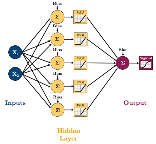
I’m going to start using ReLU as our activation function(s) and Adam as our optimizer because these are what are currently, commonly used in practice.
We are doing classification now so we’ll need to use log loss (binary cross entropy) as our loss function:

f(w) = \sum_{x,y \in D} -y log(\hat{y}) - (1-y)log(1-\hat{y})

(9)

In PyTorch, binary cross entropy loss criterion is torch.nn.BCELoss
The formula expects a “probability” which is why we add a Sigmoid function to the end of out network.

class binaryClassifier(nn.Module):
    def __init__(self, input_size, hidden_size, output_size):
        super().__init__()
        self.main = nn.Sequential(
            nn.Linear(input_size, hidden_size),
            nn.ReLU(),
            nn.Linear(hidden_size, output_size),
            nn.Sigmoid()  # <-- this will squash our output to a probability between 0 and 1
        )

    def forward(self, x):
        out = self.main(x)
        return out

BUT WAIT!
While we can do the above and then train with a torch.nn.BCELoss loss function, there’s a better way!
We can omit the Sigmoid function and just use torch.nn.BCEWithLogitsLoss (which combines a Sigmoid layer and the BCELoss)
Why would we do this? It’s numerically stable! (Did you do the log-sum-exp question in Lab 1? We use it here for stability!)
From the docs:

“This version is more numerically stable than using a plain Sigmoid followed by a BCELoss as, by combining the operations into one layer, we take advantage of the log-sum-exp trick for numerical stability.”

So actually, here’s our model (no Sigmoid layer at the end because it’s included in the loss function we’ll use):

class binaryClassifier(nn.Module):
    def __init__(self, input_size, hidden_size, output_size):
        super().__init__()
        self.main = nn.Sequential(
            nn.Linear(input_size, hidden_size),
            nn.ReLU(),
            nn.Linear(hidden_size, output_size)
        )

    def forward(self, x):
        out = self.main(x)
        return out

Let’s train the model:

def trainer(model, criterion, optimizer, dataloader, epochs=5, verbose=True):
    """Simple training wrapper for PyTorch network."""
    
    for epoch in range(epochs):
        losses = 0
        for X, y in dataloader:
            optimizer.zero_grad()       # Clear gradients w.r.t. parameters
            y_hat = model(X).flatten()  # Forward pass to get output
            loss = criterion(y_hat, y)  # Calculate loss
            loss.backward()             # Getting gradients w.r.t. parameters
            optimizer.step()            # Update parameters
            losses += loss.item()       # Add loss for this batch to running total
        if verbose: print(f"epoch: {epoch + 1}, loss: {losses / len(dataloader):.4f}")

model = binaryClassifier(2, 5, 1)
LEARNING_RATE = 0.1
criterion = torch.nn.BCEWithLogitsLoss() # loss function
optimizer = torch.optim.Adam(model.parameters(), lr=LEARNING_RATE)  # optimization algorithm
trainer(model, criterion, optimizer, dataloader, epochs=20, verbose=True)

epoch: 1, loss: 0.6842
epoch: 2, loss: 0.6534
epoch: 3, loss: 0.6097
epoch: 4, loss: 0.5676
epoch: 5, loss: 0.5343
epoch: 6, loss: 0.4916
epoch: 7, loss: 0.4410
epoch: 8, loss: 0.3871
epoch: 9, loss: 0.3299
epoch: 10, loss: 0.2833
epoch: 11, loss: 0.2467
epoch: 12, loss: 0.2135
epoch: 13, loss: 0.1992
epoch: 14, loss: 0.1889
epoch: 15, loss: 0.1800
epoch: 16, loss: 0.1695
epoch: 17, loss: 0.1698
epoch: 18, loss: 0.1687
epoch: 19, loss: 0.1541
epoch: 20, loss: 0.1510

plot_classification_2d(X, y, model)

To be clear, our model is just outputting some number between -∞ and +∞ (we aren’t applying Sigmoid), so:
- To get the probabilities we would need to pass them through a Sigmoid;
- To get classes, we can apply some threshold (usually 0.5)
For example, we would expect the point (0,0) to have a high probability and the point (-1,-1) to have a low probability:

prediction = model(torch.tensor([[0, 0], [-1, -1]], dtype=torch.float32)).detach()
print(prediction)

tensor([[  4.9344],
        [-11.3356]])

probability = nn.Sigmoid()(prediction)
print(probability)

tensor([[9.9286e-01],
        [1.1939e-05]])

classes = np.where(probability > 0.5, 1, 0)
print(classes)

[[1]
 [0]]

5.2. Multiclass Classification (Optional)¶

For multiclass classification, remember softmax?

\sigma(\vec{z})_i=\frac{e^{z_i}}{\sum_{j=1}^{K}e^{z_j}}

(10)

It basically makes sure all the outputs are probabilities between 0 and 1, and that they all sum to 1.
torch.nn.CrossEntropyLoss is a loss that combines a softmax with cross entropy loss.
Let’s try a 4-class classification problem using the following network:

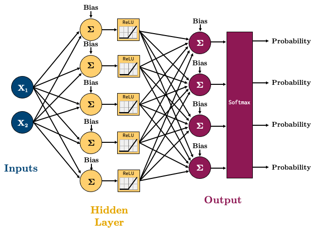
class multiClassifier(torch.nn.Module):
    def __init__(self, input_size, hidden_size, output_size):
        super().__init__()
        self.main = torch.nn.Sequential(
            torch.nn.Linear(input_size, hidden_size),
            torch.nn.ReLU(),
            torch.nn.Linear(hidden_size, output_size)
        )

    def forward(self, x):
        out = self.main(x)
        return out

X, y = make_blobs(n_samples=200, centers=4, center_box=(-1.2, 1.2), cluster_std=[0.15, 0.15, 0.15, 0.15], random_state=12345)
X_t = torch.tensor(X, dtype=torch.float32)
y_t = torch.tensor(y, dtype=torch.int64)
# Create dataloader
dataset = TensorDataset(X_t, y_t)
dataloader = DataLoader(dataset, batch_size=BATCH_SIZE, shuffle=True)
plot_classification_2d(X, y)

Let’s train this model:

model = multiClassifier(2, 5, 4)
criterion = torch.nn.CrossEntropyLoss() # loss function
optimizer = torch.optim.Adam(model.parameters(), lr=0.2)  # optimization algorithm

for epoch in range(10):
    losses = 0
    for X_batch, y_batch in dataloader:
        optimizer.zero_grad()       # Clear gradients w.r.t. parameters
        y_hat = model(X_batch)            # Forward pass to get output
        loss = criterion(y_hat, y_batch)  # Calculate loss
        loss.backward()             # Getting gradients w.r.t. parameters
        optimizer.step()            # Update parameters
        losses += loss.item()       # Add loss for this batch to running total
    print(f"epoch: {epoch + 1}, loss: {losses / len(dataloader):.4f}")

epoch: 1, loss: 1.1576
epoch: 2, loss: 0.7209
epoch: 3, loss: 0.4848
epoch: 4, loss: 0.3222
epoch: 5, loss: 0.1632
epoch: 6, loss: 0.0652
epoch: 7, loss: 0.0157
epoch: 8, loss: 0.0085
epoch: 9, loss: 0.0040
epoch: 10, loss: 0.0016

plot_classification_2d(X, y, model, transform="Softmax")

To be clear once again, our model is just outputting some number between -∞ and +∞, so:
- To get the probabilities we would need to pass them to a Softmax;
- To get classes, we need to select the largest probability.
For example, we would expect the point (-1,-1) to have a high probability of belonging to class 1, and the point (0,0) to have the highest probability of belonging to class 2.

prediction = model(torch.tensor([[-1, -1], [1,1]], dtype=torch.float32)).detach()
print(prediction)

tensor([[-27.5895,  19.3565,   1.1430, -33.1879],
        [-12.4731, -22.3387,   2.0026,  20.8498]])

Note how we get 4 predictions per data point (a prediction for each of the 4 classes)

probability = nn.Softmax(dim=1)(prediction)
print(probability)

tensor([[4.0889e-21, 1.0000e+00, 1.2302e-08, 1.5144e-23],
        [3.3731e-15, 1.7517e-19, 6.5275e-09, 1.0000e+00]])

The predictions should now sum to 1:

probability.sum(dim=1)

tensor([1., 1.])

We can get the class with maximum probability using argmax():

classes = probability.argmax(dim=1)
print(classes)

tensor([1, 3])

Lecture Exercise: True/False Questions¶

Answer True/False for the following:

Neural networks can be used for both regression and classification. (True)
For fully connected neural networks, the number of parameters $\geq$ the number of features. (True)
Neural networks are parametric models. (True)
Any neural network with 3 hidden layers will have more parameters than any neural network with 2 hidden layers. (False)
The architecture of a neural network (number of hidden layers and hidden nodes) is a hyperparameter. (True)
Like linear regression or logistic regression, with neural networks we can interpret each feature’s weight value as a measure of the feature’s importance. (False)

The Lecture in Three Conjectures¶

PyTorch is a neural network software based on “tensors” (like NumPy arrays on steroids).
Neural Networks are simply:
- Composed of an input layer, 1 or more hidden layers, and an output layer, each with 1 or more nodes.
- The number of nodes in the Input/Output layers is defined by the problem/data. Hidden layers can have an arbitrary number of nodes.
- Activation functions in the hidden layers help us model non-linear data.
- Feed-forward neural networks are just a combination of simple linear and non-linear operations.
Activation functions allow the network to learn non-linear function