
Example Notebook#
Mahmood Amintoosi
Computer Science Dept, Ferdowsi University of Mashhad
You can also create content with Jupyter Notebooks. This means that you can include code blocks and their outputs in your book. In this notebook, we show some examples of loading and plotting data. Check this documentation about how to write executable content.
Show code cell source
# Import packages
import pandas as pd
import plotly.express as px
import seaborn as sns
Load data#
You can put your data at the same directory as the notebook file and then use pandas to load the data.
# Load the Iris flower dataset using pandas
df = pd.read_csv("iris_data.csv")
df
| sepal_length | sepal_width | petal_length | petal_width | species | species_id | |
|---|---|---|---|---|---|---|
| 0 | 5.1 | 3.5 | 1.4 | 0.2 | setosa | 1 |
| 1 | 4.9 | 3.0 | 1.4 | 0.2 | setosa | 1 |
| 2 | 4.7 | 3.2 | 1.3 | 0.2 | setosa | 1 |
| 3 | 4.6 | 3.1 | 1.5 | 0.2 | setosa | 1 |
| 4 | 5.0 | 3.6 | 1.4 | 0.2 | setosa | 1 |
| ... | ... | ... | ... | ... | ... | ... |
| 145 | 6.7 | 3.0 | 5.2 | 2.3 | virginica | 3 |
| 146 | 6.3 | 2.5 | 5.0 | 1.9 | virginica | 3 |
| 147 | 6.5 | 3.0 | 5.2 | 2.0 | virginica | 3 |
| 148 | 6.2 | 3.4 | 5.4 | 2.3 | virginica | 3 |
| 149 | 5.9 | 3.0 | 5.1 | 1.8 | virginica | 3 |
150 rows × 6 columns
Plot data#
We set the repository in a way that you can use Plotly for interactive visualizations. For more information, check this documentation.
# Plot the Iris dataset using Plotly
g1 = px.scatter_3d(df,
                   x="sepal_width",
                   y="sepal_length",
                   z="petal_width",
                   color="species",
                   size="petal_length",
                   opacity=0.6,
                   size_max=30,
                   height=700)
g1
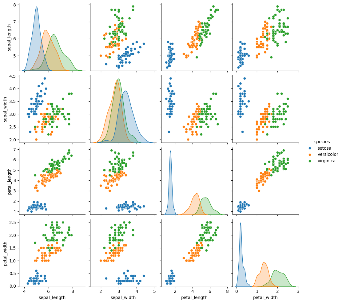
You can also plot the data using static visualizations, such as the seaborn library.
# Plot the Iris dataset using seaborn
g2 = sns.pairplot(df.drop("species_id", axis=1),
                  hue='species')
g2
<seaborn.axisgrid.PairGrid at 0x17ab16a64e0>
Math Formulas with \(\LaTeX\)#
Univariate Normal Density:
\[ p(x) = \frac{1}{\sqrt{2\pi}\sigma} \exp\left[-\frac{1}{2}\left(\frac{x-\mu}{\sigma}\right)^2\right] \]
For which the expected value of \(x\) (an average, here taken over the feature space) is:
and where the expected squared deviation or variance is:
The univariate normal density is completely specified by two parameters: its mean \(\mu\) and variance \(\sigma^2\). For simplicity, we often abbreviate \(p(x)\) by writing \(p(x) \sim N(\mu, \sigma^2)\) to say that \(x\) is distributed normally with mean \(\mu\) and variance \(\sigma^2\). Samples from normal distributions tend to cluster about the mean, with a spread related to the standard deviation \(\sigma\) (See Chapter 2 of Pattern Classification [DHS00]).