Gaussian Mixture Model, Part 2

The contents of this section are derived from Chapter 13 of Data Mining and Machine Learning by Mohammed J. Zaki and Wagner Meira Jr. (2020) Zaki & Meira (2020).

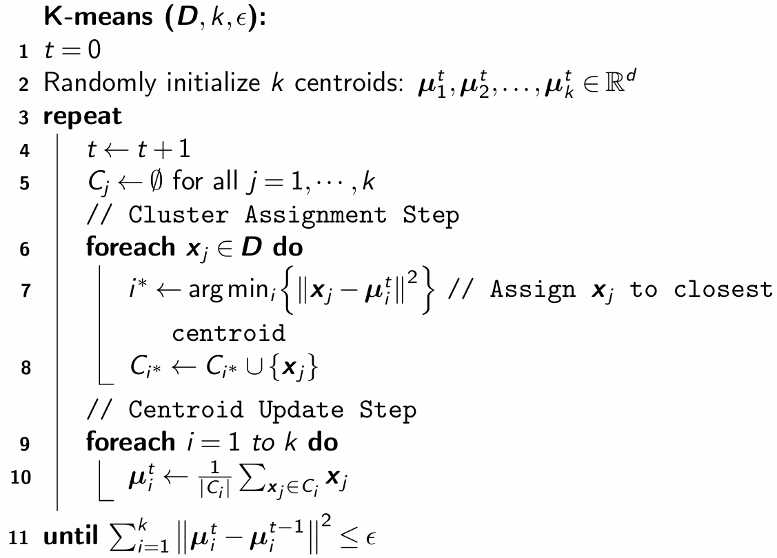
K-means Algorithm: Review¶

The sum of squared errors scoring function is defined as

The goal is to find the clustering that minimizes the SSE score:

K-means employs a greedy iterative approach to find a clustering that minimizes the SSE objective. As such, it can converge to a local optimum instead of a globally optimal clustering.

K-means Algorithm: Steps¶

K-means initializes the cluster means by randomly generating $k$ points in the data space. Each iteration consists of two steps:

1. Cluster Assignment: Each point $\mathbf{x}_{j} \in \mathbf{D}$ is assigned to the closest mean, inducing a clustering with each cluster $C_i$ comprising points closest to $\mathbf{\mu}_i$:

   $$i^* = \arg \min_{i=1}^k \Bigl\{\|\mathbf{x}_{j} - \mathbf{\mu}_i\|^2\Bigr\}$$

   (3)

2. Centroid Update: New mean values are computed for each cluster from the points in $C_i$.

These steps iterate until convergence to a fixed point or local minimum.

K-Means Algorithm¶

Expectation-Maximization Clustering¶

Let $X_a$ denote the random variable corresponding to the $a^{th}$ attribute. Let $\mathbf{X} = (X_1, X_2, \dots, X_d)$ denote the vector random variable across the $d$ attributes, with $\mathbf{x}_{j}$ being a data sample from $\mathbf{X}$.

We assume each cluster $C_i$ is characterized by a multivariate normal distribution:

where $\mathbf{\mu}_i \in \mathbb{R}^d$ is the cluster mean and $\mathbf{\Sigma}_i \in \mathbb{R}^{d \times d}$ is the covariance matrix.

The probability density function of $\mathbf{X}$ is given as a Gaussian mixture model over all the $k$ clusters:

where the prior probabilities $P(C_i)$ are called the mixture parameters, which must satisfy the condition:

Maximum Likelihood Estimation¶

We write the set of all model parameters compactly as:

Given the dataset $\mathbf{D}$, the likelihood of $\mathbf{\theta}$ is:

MLE chooses parameters $\mathbf{\theta}$ to maximize likelihood:

where the log-likelihood function is:

Maximizing Log-Likelihood with Expectation-Maximization (EM)¶

Directly maximizing the log-likelihood over $\mathbf{\theta}$ is difficult because of the summation inside the logarithm:

If the likelihood function involved only a single Gaussian, direct differentiation would be straightforward. However, in a Gaussian mixture model, the presence of multiple Gaussians inside the summation complicates differentiation. Since each data point $\mathbf{x}_j$ does not belong to one cluster deterministically but instead has a probability of belonging to multiple clusters, it is difficult to solve for the parameters analytically.

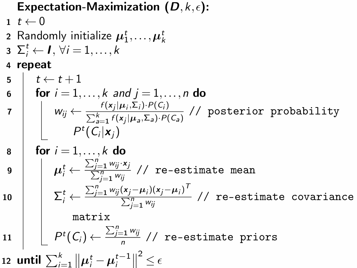
How does EM help?¶

Expectation-Maximization provides a structured approach to indirectly maximize the likelihood by introducing latent variables—the cluster assignments $w_{ij} = P(C_i | \mathbf{x}_j)$. The Expectation step computes these probabilities, effectively estimating the hidden memberships, while the Maximization step updates the parameters using these weights.

By iterating between these steps, EM avoids the complexity of differentiating the nested sum-log expression directly, making parameter estimation feasible.

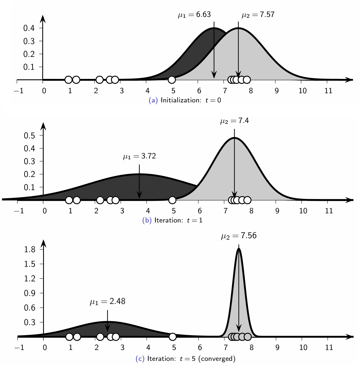
Expectation-Maximization for Gaussian Mixture Models¶

1D Case: Univariate Normal Clustering¶

Let $\mathbf{D}$ comprise a single attribute $X$, where each point $x_{j} \in \mathbb{R}$ is a random sample from $X$. The mixture model uses univariate normal distributions for each cluster:

where the cluster parameters include $\mu_{i}$ (mean), $\sigma_{i}^2$ (variance), and $P(C_i)$ (prior probability).

Initialization¶

Each cluster $C_i$ (for $i = 1, 2, \dots, k$) is randomly initialized with parameters $\mu_{i}$, $\sigma_{i}^2$, and $P(C_i)$.

Expectation Step¶

Given the mean $\mu_i$, variance $\sigma_i^2$, and prior probability $P(C_i)$ for each cluster, the cluster posterior probability is computed using Bayes’ theorem:

Maximization Step¶

Using $w_{ij}$, the updated cluster parameters are computed as follows:

• Mean update (weighted average of points):

  $$\mu_{i} = \frac{\sum_{j=1}^n w_{ij} \cdot x_{j}} {\sum_{j=1}^n w_{ij}}$$

  (14)

• Variance update (weighted variance of points):

  $$\sigma_{i}^{2} = \frac{\sum_{j=1}^n w_{ij}(x_{j}-\mu_{i})^2} {\sum_{j=1}^n w_{ij}}$$

  (15)

• Prior probability update (fraction of weights contributing to the cluster):

  $$P(C_{i}) = \frac{\sum_{j=1}^n w_{ij}}{n}$$

  (16)

Multivariate Case: Full Covariance Gaussian Mixture Model¶

In the multivariate case, each cluster $C_i$ is modeled by a multivariate normal distribution, extending beyond the 1D case:

where $\mathbf{\mu}_i \in \mathbb{R}^d$ is the cluster mean and $\mathbf{\Sigma}_i \in \mathbb{R}^{d \times d}$ is the covariance matrix.

Expectation Step (Multivariate)¶

Similar to the univariate case, the cluster posterior probability is computed using Bayes’ theorem:

Maximization Step (Multivariate)¶

• Mean update (weighted average of points):

  $$\mathbf{\mu}_{i} = \frac{\sum_{j=1}^n P(C_i | \mathbf{x}_j) \cdot \mathbf{x}_{j}} {\sum_{j=1}^n P(C_i | \mathbf{x}_j)}$$

  (19)

• Covariance update (weighted covariance matrix across dimensions):

  $$\mathbf{\Sigma}_{i} = \frac{\sum_{j=1}^n P(C_i | \mathbf{x}_j) (\mathbf{x}_j - \mathbf{\mu}_i)(\mathbf{x}_j - \mathbf{\mu}_i)^T} {\sum_{j=1}^n P(C_i | \mathbf{x}_j)}$$

  (20)

• Prior probability update (fraction of total contribution to the cluster):

  $$P(C_{i}) = \frac{\sum_{j=1}^n P(C_i | \mathbf{x}_j)}{n}$$

  (21)

Expectation-Maximization Clustering Algorithm¶

K-Means as a Special Case of Expectation-Maximization (EM)¶

K-means can be viewed as a simplified version of the Expectation-Maximization (EM) algorithm, where cluster assignments are deterministic rather than probabilistic. Specifically, in K-means, each data point $\mathbf{x}_{j}$ belongs exclusively to one cluster based on the minimum squared distance to the cluster centroid:

The posterior probability of cluster assignment is calculated using Bayes’ theorem:

Since K-means deterministically assigns each point to exactly one cluster, this simplifies to the following cases:

• If $P(\mathbf{x}_{j} | C_i) = 0$, then $P(C_i | \mathbf{x}_{j}) = 0$.

• If $P(\mathbf{x}_{j} | C_i) = 1$, then for all $a \neq i$, we have $P(\mathbf{x}_{j} | C_a) = 0$, so:

  $$P(C_i | \mathbf{x}_{j}) = \frac{1 \cdot P(C_i)}{1 \cdot P(C_i)} = 1.$$

  (24)

Thus, in K-means, cluster membership is binary:

Unlike EM, which incorporates covariance matrices to model cluster distributions, K-means only estimates the cluster centroids $\mathbf{\mu}_i$ and the cluster proportions $P(C_i)$.