Introduction to Network Analysis with NetworkX - Mathematical Foundations of Data Science

Graph Data Structures and Operations¶

In this Jupyter notebook, we will explore the basics of graph data structures and operations using the NetworkX library in Python. NetworkX is a powerful library for creating, manipulating, and studying the structure and dynamics of complex networks.

We will start by creating simple directed and undirected graphs, and then explore some basic graph operations, such as breadth-first search (BFS).

Importing Necessary Libraries¶

import networkx as nx
import matplotlib.pyplot as plt

Creating an un-directed Graph¶

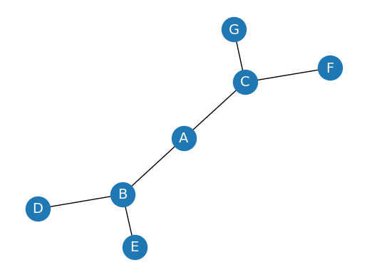
First, let’s create a simple un-directed graph and visualize it:


G = nx.Graph()
G.add_edges_from([('A', 'B'), ('A', 'C'), ('B', 'D'), ('B', 'E'), ('C', 'F'), ('C', 'G')])

plt.axis('off')
nx.draw_networkx(G,
                 pos=nx.spring_layout(G, seed=0),
                 node_size=600,
                 cmap='coolwarm',
                 font_size=14,
                 font_color='white'
                 )

f:\conda\envs\pth-gpu\lib\site-packages\networkx\drawing\nx_pylab.py:433: UserWarning: No data for colormapping provided via 'c'. Parameters 'cmap' will be ignored
  node_collection = ax.scatter(

Creating a Directed Graph¶

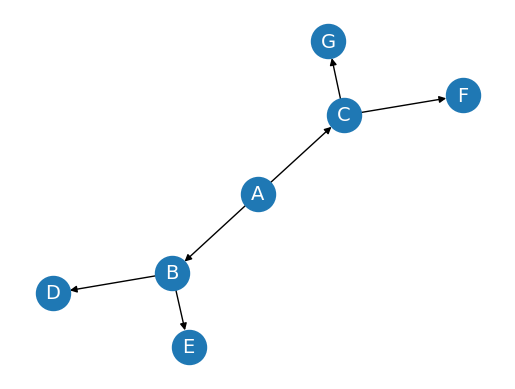
Now, let’s create a simple directed graph (DiGraph) and visualize it:

DG = nx.DiGraph()
DG.add_edges_from([('A', 'B'), ('A', 'C'), ('B', 'D'), ('B', 'E'), ('C', 'F'), ('C', 'G')])

plt.axis('off')
nx.draw_networkx(DG,
                 pos=nx.spring_layout(G, seed=0),
                 node_size=600,
                 cmap='coolwarm',
                 font_size=14,
                 font_color='white'
                 )

Create a weighted graph WG and visualize it with edge weights¶

WG = nx.Graph()
WG.add_edges_from([('A', 'B', {"weight": 10}), ('A', 'C', {"weight": 20}), ('B', 'D', {"weight": 30}), ('B', 'E', {"weight": 40}), ('C', 'F', {"weight": 50}), ('C', 'G', {"weight": 60})])
labels = nx.get_edge_attributes(WG, "weight")

plt.axis('off')
nx.draw_networkx(WG,
                 pos=nx.spring_layout(G, seed=0),
                 node_size=600,
                 cmap='coolwarm',
                 font_size=14,
                 font_color='white'
                 )
nx.draw_networkx_edge_labels(WG, pos=nx.spring_layout(G, seed=0), edge_labels=labels)

{('A', 'B'): Text(-0.17063150397490368, -0.25785521234238246, '10'),
 ('A', 'C'): Text(0.16908485308194388, 0.2584267536065791, '20'),
 ('B', 'D'): Text(-0.5751319512575159, -0.5819114840781281, '30'),
 ('B', 'E'): Text(-0.3070875406419613, -0.7577069745265291, '40'),
 ('C', 'F'): Text(0.5743060275721562, 0.5815239318372771, '50'),
 ('C', 'G'): Text(0.3081446719975651, 0.7583070963940803, '60')}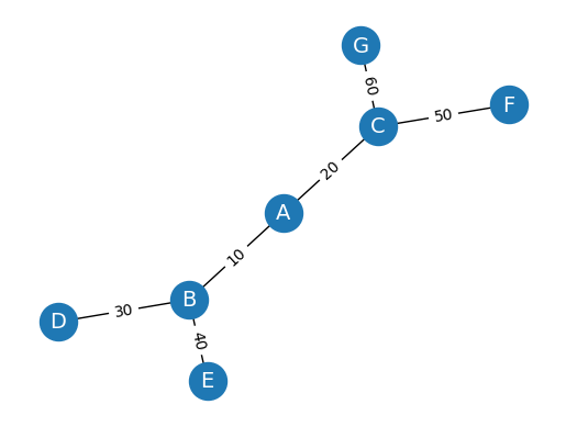

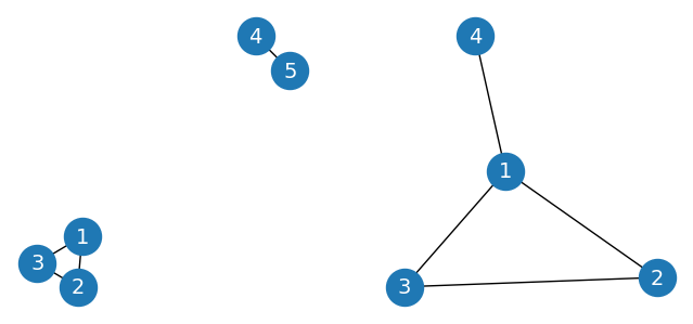
Check the connectivity of two different graphs¶

G1 = nx.Graph()
G1.add_edges_from([(1, 2), (2, 3), (3, 1), (4, 5)])
print(f"Is graph 1 connected? {nx.is_connected(G1)}")

G2 = nx.Graph()
G2.add_edges_from([(1, 2), (2, 3), (3, 1), (1, 4)])
print(f"Is graph 2 connected? {nx.is_connected(G2)}")

Is graph 1 connected? False
Is graph 2 connected? True

Visualize the two graphs side-by-side¶

plt.figure(figsize=(8,8))
plt.subplot(221)
plt.axis('off')
nx.draw_networkx(G1,
                 pos=nx.spring_layout(G1, seed=0),
                 node_size=600,
                 cmap='coolwarm',
                 font_size=14,
                 font_color='white'
                 )
plt.subplot(222)
plt.axis('off')
nx.draw_networkx(G2,
                 pos=nx.spring_layout(G2, seed=0),
                 node_size=600,
                 cmap='coolwarm',
                 font_size=14,
                 font_color='white'
                 )

Calculate degree of node A for an undirected graph G and a directed graph DG¶

G = nx.Graph()
G.add_edges_from([('A', 'B'), ('A', 'C'), ('B', 'D'), ('B', 'E'), ('C', 'F'), ('C', 'G')])
print(f"deg(A) = {G.degree['A']}")

DG = nx.DiGraph()
DG.add_edges_from([('A', 'B'), ('A', 'C'), ('B', 'D'), ('B', 'E'), ('C', 'F'), ('C', 'G')])
print(f"deg^-(A) = {DG.in_degree['A']}")
print(f"deg^+(A) = {DG.out_degree['A']}")

deg(A) = 2
deg^-(A) = 0
deg^+(A) = 2

plt.axis('off')
nx.draw_networkx(G,
                 pos=nx.spring_layout(G, seed=0),
                 node_size=600,
                 cmap='coolwarm',
                 font_size=14,
                 font_color='white'
                 )

Calculate degree centrality measures for an undirected graph G

print(f"Degree centrality      = {nx.degree_centrality(G)}")
print(f"Closeness centrality   = {nx.closeness_centrality(G)}")
print(f"Betweenness centrality = {nx.betweenness_centrality(G)}")

Degree centrality      = {'A': 0.3333333333333333, 'B': 0.5, 'C': 0.5, 'D': 0.16666666666666666, 'E': 0.16666666666666666, 'F': 0.16666666666666666, 'G': 0.16666666666666666}
Closeness centrality   = {'A': 0.6, 'B': 0.5454545454545454, 'C': 0.5454545454545454, 'D': 0.375, 'E': 0.375, 'F': 0.375, 'G': 0.375}
Betweenness centrality = {'A': 0.6, 'B': 0.6, 'C': 0.6, 'D': 0.0, 'E': 0.0, 'F': 0.0, 'G': 0.0}

Represent graphs using different data structures (adjacency matrix, edge list, adjacency list)

adj = [[0,1,1,0,0,0,0],
       [1,0,0,1,1,0,0],
       [1,0,0,0,0,1,1],
       [0,1,0,0,0,0,0],
       [0,1,0,0,0,0,0],
       [0,0,1,0,0,0,0],
       [0,0,1,0,0,0,0]]

edge_list = [(0, 1), (0, 2), (1, 3), (1, 4), (2, 5), (2, 6)]

adj_list = {
    0: [1, 2],
    1: [0, 3, 4],
    2: [0, 5, 6],
    3: [1],
    4: [1],
    5: [2],
    6: [2]
}

Creating an Undirected Graph and Performing Breadth-First Search (BFS)¶

Next, let’s create an undirected graph G and perform a BFS traversal starting from node ‘A’:

G = nx.Graph()
G.add_edges_from([('A', 'B'), ('A', 'C'), ('B', 'D'), ('B', 'E'), ('C', 'F'), ('C', 'G')])

def bfs(graph, node):
    visited, queue = [node], [node]

    while queue:
        node = queue.pop(0)
        for neighbor in graph[node]:
            if neighbor not in visited:
                visited.append(neighbor)
                queue.append(neighbor)

    return visited

bfs(G, 'A')

['A', 'B', 'C', 'D', 'E', 'F', 'G']

Perform Depth-First Search (DFS) on an undirected graph G

visited = []

def dfs(visited, graph, node):
    if node not in visited:
        visited.append(node)
        for neighbor in graph[node]:
            visited = dfs(visited, graph, neighbor)

    return visited

dfs(visited, G, 'A')

['A', 'B', 'D', 'E', 'C', 'F', 'G']

Erdős-Rényi Model¶

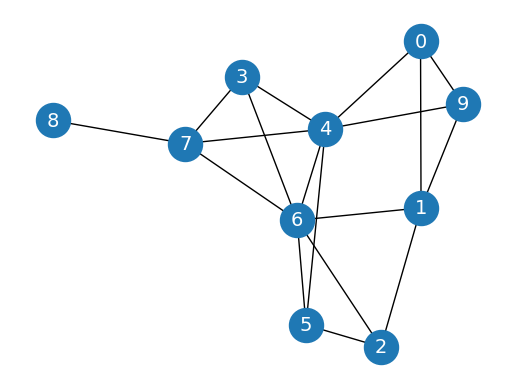
nx.erdos_renyi_graph is a function from the NetworkX library in Python that generates a random graph based on the Erdős-Rényi model. This model is one of the simplest and most widely studied random graph models.

Overview of the Erdős-Rényi Model¶

There are two primary formulations of the Erdős-Rényi model:

G(n, p): In this model, a graph is constructed by adding nodes one at a time (where ( n ) is the total number of nodes). Each possible edge between any pair of nodes is included independently with a probability ( p ).
G(n, m): In this model, ( n ) nodes are connected by creating exactly ( m ) edges chosen uniformly at random from all possible edges that could exist between the nodes.

The Erdős-Rényi random graphs are often used in various fields, including:

Network theory: To study the properties of random graphs.
Computer science: In algorithms related to networks and to simulate networks with random connections.

Random graphs can help researchers understand the behavior of more complex structures and networks in real-world applications.

import networkx as nx
import matplotlib.pyplot as plt
import numpy as np

# Create a graph
G = nx.erdos_renyi_graph(10, 0.3, seed=1, directed=False)

# Plot graph
plt.figure()
plt.axis('off')
nx.draw_networkx(G,
                 pos=nx.spring_layout(G, seed=0),
                 node_size=600,
                 cmap='coolwarm',
                 font_size=14,
                 font_color='white'
                 )