Linear models

Linear models
Basics of modeling, optimization, and regularization
Mahmood Amintoosi, Spring 2026
Computer Science Dept, Ferdowsi University of Mashhad
I should mention that the original material of this course was from Open Machine Learning Course, by Joaquin Vanschoren and others.
Source
# Auto-setup when running on Google Colab
import os
if 'google.colab' in str(get_ipython()) and not os.path.exists('/content/machine-learning'):
    !git clone -q https://github.com/fum-cs/machine-learning.git /content/machine-learning
    !pip --quiet install -r /content/machine-learning/requirements_colab.txt
    %cd machine-learning/notebooks

# Global imports and settings
%matplotlib inline
from preamble import *
interactive = False # Set to True for interactive plots
if interactive:
    fig_scale = 0.5
    plt.rcParams.update(print_config)
else: # For printing
    fig_scale = 0.3
    plt.rcParams.update(print_config)
Notation and Definitions
A scalar is a simple numeric value, denoted by an italic letter:
A vector is a 1D ordered array of n scalars, denoted by a bold letter:
denotes the th element of a vector, thus .
Note: some other courses use notation
A set is an unordered collection of unique elements, denote by caligraphic capital:
A matrix is a 2D array of scalars, denoted by bold capital:
denotes the th row of the matrix
denotes the th column
denotes the element in the th row, th column, thus
, an matrix, can represent data points in a -dimensional space
Every row is a vector that can represent a point in an p-dimensional space, given a basis.
The standard basis for a Euclidean space is the set of unit vectors
E.g. if
Source
X = np.array([[3.24 , 1.2 ],[2.24, 0.2],[3.0 , 0.6 ]])
fig = plt.figure(figsize=(5*fig_scale,4*fig_scale))
plt.scatter(X[:,0],X[:,1])
for i in range(3):
plt.annotate(i, (X[i,0]+0.02, X[i,1]))A tensor is an k-dimensional array of data, denoted by an italic capital:
k is also called the order, degree, or rank
denotes the element or sub-tensor in the corresponding position
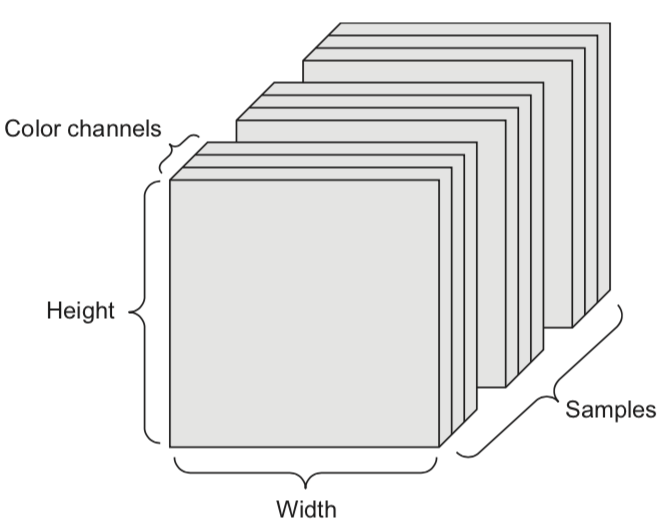
A set of color images can be represented by:
a 4D tensor (sample x height x width x color channel)
a 2D tensor (sample x flattened vector of pixel values)
Basic operations
Sums and products are denoted by capital Sigma and capital Pi:
Operations on vectors are element-wise: e.g.
Dot product
Matrix product
A function relates an input element to an output
It has a local minimum at if in interval
It has a global minimum at if for any value for
A vector function consumes an input and produces a vector:
returns the largest value f(x) for any x
returns the element x that maximizes f(x)
Gradients
A derivative of a function describes how fast grows or decreases
The process of finding a derivative is called differentiation
Derivatives for basic functions are known
For non-basic functions we use the chain rule:
A function is differentiable if it has a derivative in any point of it’s domain
It’s continuously differentiable if is a continuous function
We say is smooth if it is infinitely differentiable, i.e., all exist
A gradient is the derivative of a function in multiple dimensions
It is a vector of partial derivatives:
E.g.
Example:
Evaluated at point (-4,1):
These are the slopes at point (-4,1) in the direction of and respectively
Source
from mpl_toolkits import mplot3d
import ipywidgets as widgets
from ipywidgets import interact, interact_manual

# f = -(x0^2 + x1^2)
def g_f(x0, x1):
    return -(x0 ** 2 + x1 ** 2)
def g_dfx0(x0):
    return -2 * x0
def g_dfx1(x1):
    return -2 * x1

@interact
def plot_gradient(rotation=(0,240,10)):
    # plot surface of f
    fig = plt.figure(figsize=(12*fig_scale,5*fig_scale))
    ax = plt.axes(projection="3d")
    x0 = np.linspace(-6, 6, 30)
    x1 = np.linspace(-6, 6, 30)
    X0, X1 = np.meshgrid(x0, x1)
    ax.plot_surface(X0, X1, g_f(X0, X1), rstride=1, cstride=1,
                    cmap='winter', edgecolor='none',alpha=0.3)

    # choose point to evaluate: (-4,1)
    i0 = -4
    i1 = 1
    iz = np.linspace(g_f(i0,i1), -82, 30)
    ax.scatter3D(i0, i1, g_f(i0,i1), c="k", s=20*fig_scale,label='($i_0$,$i_1$) = (-4,1)')
    ax.plot3D([i0]*30, [i1]*30, iz, linewidth=1*fig_scale, c='silver', linestyle='-')
    ax.set_zlim(-80,0)

    # plot intersects
    ax.plot3D(x0,[1]*30,g_f(x0, 1),linewidth=3*fig_scale,alpha=0.9,label='$f(x_0,i_1)$',c='r',linestyle=':')
    ax.plot3D([-4]*30,x1,g_f(-4, x1),linewidth=3*fig_scale,alpha=0.9,label='$f(i_0,x_1)$',c='b',linestyle=':')

    # df/dx0 is slope of line at the intersect point
    x0 = np.linspace(-8, 0, 30)
    ax.plot3D(x0,[1]*30,g_dfx0(i0)*x0-g_f(i0,i1),linewidth=3*fig_scale,label=r'$\frac{\partial f}{\partial x_0}(i_0,i_1) x_0 + f(i_0,i_1)$',c='r',linestyle='-')
    ax.plot3D([-4]*30,x1,g_dfx1(i1)*x1+g_f(i0,i1),linewidth=3*fig_scale,label=r'$\frac{\partial f}{\partial x_1}(i_0,i_1) x_1 + f(i_0,i_1)$',c='b',linestyle='-')

    ax.set_xlabel('x0', labelpad=-4/fig_scale)
    ax.set_ylabel('x1', labelpad=-4/fig_scale)
    ax.get_zaxis().set_ticks([])
    ax.view_init(30, rotation) # Use this to rotate the figure
    ax.legend()
    box = ax.get_position()
    ax.set_position([box.x0, box.y0, box.width * 0.8, box.height])
    ax.legend(loc='center left', bbox_to_anchor=(1, 0.5))
    ax.tick_params(axis='both', width=0, labelsize=10*fig_scale, pad=-6)

    plt.tight_layout()
plt.show()Source
if not interactive:
plot_gradient(rotation=120)Distributions and Probabilities
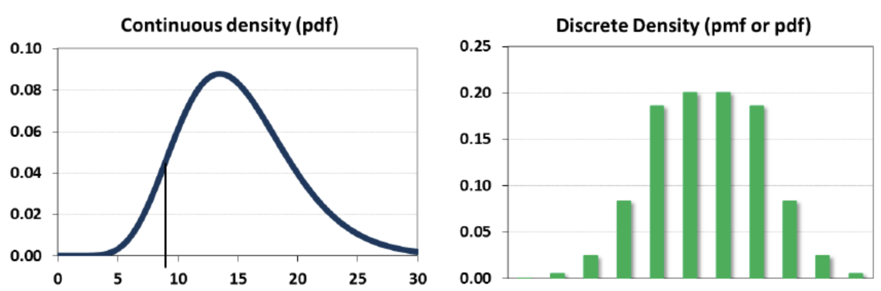
The normal (Gaussian) distribution with mean and standard deviation is noted as
A random variable can be continuous or discrete
A probability distribution of a continuous variable : probability density function (pdf)
The expectation is given by
A probability distribution of a discrete variable: probability mass function (pmf)
The expectation (or mean)
Linear models
Linear models make a prediction using a linear function of the input features
Learn from , given a loss function :
Many algorithms with different : Least squares, Ridge, Lasso, Logistic Regression, Linear SVMs,...
Can be very powerful (and fast), especially for large datasets with many features.
Can be generalized to learn non-linear patterns: Generalized Linear Models
Features can be augmentented with polynomials of the original features
Features can be transformed according to a distribution (Poisson, Tweedie, Gamma,...)
Some linear models (e.g. SVMs) can be kernelized to learn non-linear functions
Linear models for regression
Prediction formula for input features x:
... usually called weights or coefficients , the bias or intercept
Assumes that errors are
Source
from sklearn.linear_model import LinearRegression
from sklearn.model_selection import train_test_split
from mglearn.datasets import make_wave

Xw, yw = make_wave(n_samples=60)
Xw_train, Xw_test, yw_train, yw_test = train_test_split(Xw, yw, random_state=42)

line = np.linspace(-3, 3, 100).reshape(-1, 1)

lr = LinearRegression().fit(Xw_train, yw_train)
print("w_1: %f  w_0: %f" % (lr.coef_[0], lr.intercept_))

plt.figure(figsize=(6*fig_scale, 3*fig_scale))
plt.plot(line, lr.predict(line), lw=fig_scale)
plt.plot(Xw_train, yw_train, 'o', c='b')
#plt.plot(X_test, y_test, '.', c='r')
ax = plt.gca()
ax.grid(True)
ax.set_ylim(-2, 2)
ax.set_xlabel('x')
ax.set_ylabel('y')
ax.legend(["model", "training data"], loc="best");
w_1: 0.393906 w_0: -0.031804
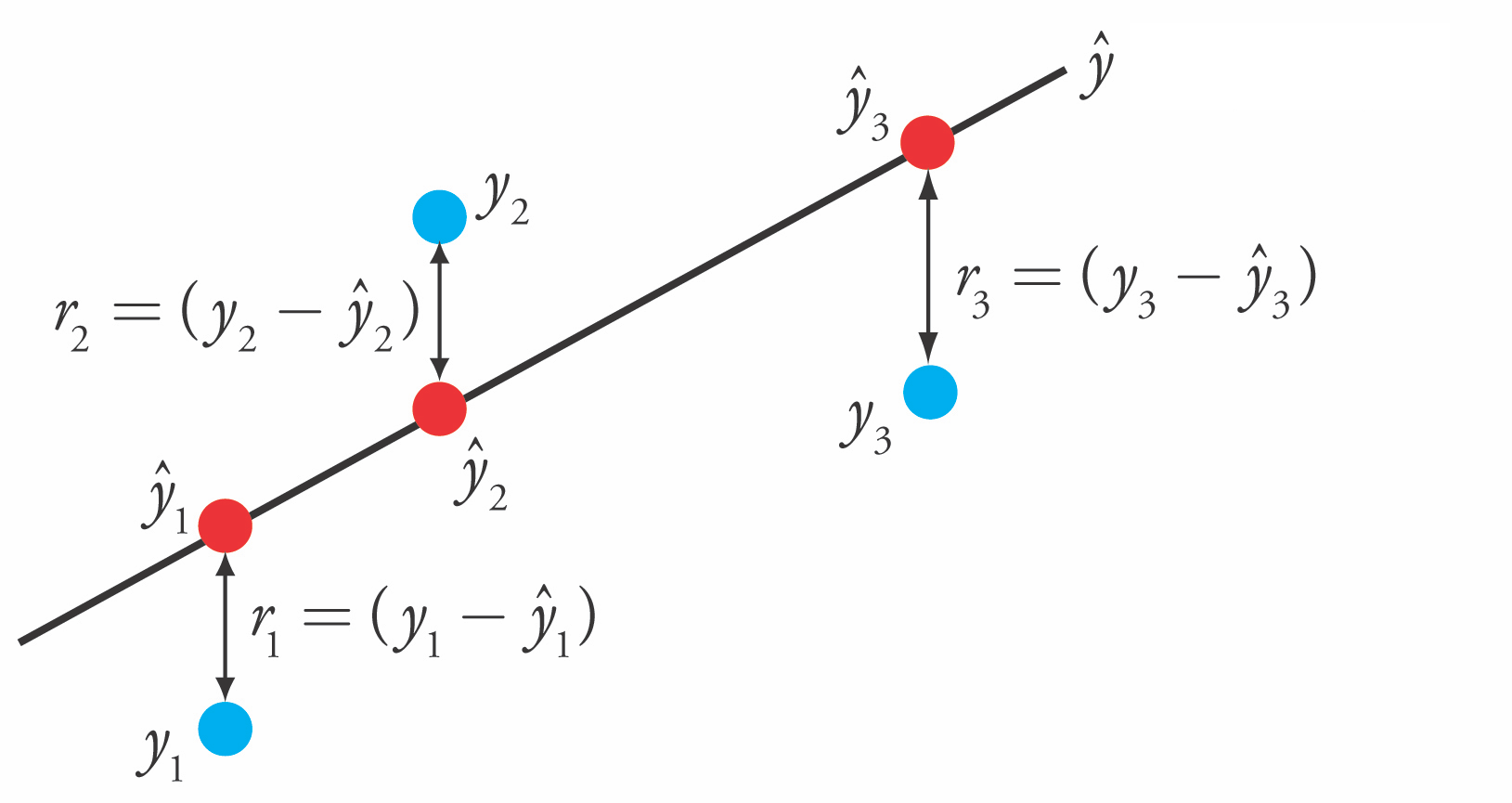
Linear Regression (aka Ordinary Least Squares)
Loss function is the sum of squared errors (SSE) (or residuals) between predictions (red) and the true regression targets (blue) on the training set.
Solving ordinary least squares
Closed-Form Solution
Convex optimization problem with unique closed-form solution:
If we have:
then can be considered as dot product of two vectors:
If instance is shown by
then:
Loss: Sum of Squared Error:
where:
We Know that (See Matrix Calculus in Wikipedia):
and if be a symmetric matrix:
Hence:
Set the derivative equal to zero:
Some notes about Closed-Form Solution
The unique closed-form solution:
Where X has rows, features, hence has dimensionality
Notes:
Slow. Time complexity is quadratic in number of features:
Only works if , is Singular When , making OLS’s undefined.
The closed-form solution of Ordinary Least Squares (OLS) is highly prone to overfitting, especially when applied to small or highly correlated datasets.
Large coefficients: In the absence of regularization, weights can grow excessively, leading to unstable predictions.
Sensitive to input variations: Small changes in may result in disproportionately large shifts in the output , making the model unreliable.
No direct hyperparameter control: Unlike Gradient Descent, OLS lacks tuning mechanisms such as learning rate or regularization strength.
Gradient Descent
More efficient for large-scale or high-dimensional datasets.
Preferred when computing is infeasible or excessively time-consuming due to large or .
Offers multiple tunable settings to control the learning process, including:
Learning Rate: Adjusts update speed to balance stability and convergence.
Regularization: Options like L1, L2, or Elastic Net mitigate overfitting.
Batch Size: Influences computational efficiency (Stochastic, Mini-batch, Full-batch).
Iterations: Determines the number of passes over the dataset.
Momentum & Decay: Helps stabilize and refine the learning trajectory.
Source
import numpy as np

# Example with n=2, p=3 (n < p)
X = np.array([[1, 2, 3],
              [4, 5, 6]])  # 2x3 matrix (n=2, p=3)

# Compute X^T X
XTX = np.dot(X.T, X)  # or X.T @ X

print("X (design matrix):")
print(X)
print("\nX^T X (Gram matrix):")
print(XTX)

# Check singularity
rank_X = np.linalg.matrix_rank(X)
rank_XTX = np.linalg.matrix_rank(XTX)
is_singular = rank_XTX < XTX.shape[0]  # True if singular

print("\nRank of X:", rank_X)
print("Rank of X^T X:", rank_XTX)
print("Is X^T X singular?", is_singular)

# Attempt to invert (will fail)
try:
    np.linalg.inv(XTX)
except np.linalg.LinAlgError:
    print("\nError: X^T X is singular and cannot be inverted (as expected when n < p).")
X (design matrix):
[[1 2 3]
[4 5 6]]
X^T X (Gram matrix):
[[17 22 27]
[22 29 36]
[27 36 45]]
Rank of X: 2
Rank of X^T X: 2
Is X^T X singular? True
Error: X^T X is singular and cannot be inverted (as expected when n < p).
Gradient Descent
Start with an initial, random set of weights:
Given a differentiable loss function (e.g. ), compute
For least squares:
If feature is associated with big errors, the gradient wrt will be large
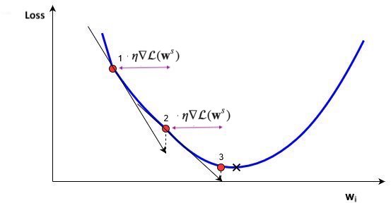
Update all weights slightly (by step size or learning rate ) in ‘downhill’ direction.
Basic update rule (step s):
Important hyperparameters
Learning rate
Too small: slow convergence. Too large: possible divergence
Maximum number of iterations
Too small: no convergence. Too large: wastes resources
Learning rate decay with decay rate
E.g. exponential (), inverse-time (),...
Many more advanced ways to control learning rate (see later)
Adaptive techniques: depend on how much loss improved in previous step
Source
import math
# Some convex function to represent the loss
def l_fx(x):
    return (x * 4)**2
# Derivative to compute the gradient
def l_dfx0(x0):
    return 8 * x0

@interact
def plot_learning_rate(learn_rate=(0.01,0.4,0.01), exp_decay=False):
    w = np.linspace(-1,1,101)
    f = [l_fx(i) for i in w]
    w_current = -0.75
    learn_rate_current = learn_rate
    fw = [] # weight values
    fl = [] # loss values
    for i in range(10):
        fw.append(w_current)
        fl.append(l_fx(w_current))
        # Decay
        if exp_decay:
            learn_rate_current = learn_rate * math.exp(-0.3*i)
        # Update rule
        w_current = w_current - learn_rate_current * l_dfx0(w_current)
    fig, ax = plt.subplots(figsize=(5*fig_scale,3*fig_scale))
    ax.set_xlabel('w')
    ax.set_xticks([])
    ax.set_ylabel('loss')
    ax.plot(w, f, lw=2*fig_scale, ls='-', c='k', label='Loss')
    ax.plot(fw, fl, '--bo', lw=2*fig_scale, markersize=3)
    plt.ylim(-1,16)
    plt.xlim(-1,1)
Output
Source
if not interactive:
plot_learning_rate(learn_rate=0.21, exp_decay=False)Source
import tensorflow as tf
# import tensorflow_addons as tfa

# Toy surface
def f(x, y):
    return (1.5 - x + x*y)**2 + (2.25 - x + x*y**2)**2 + (2.625 - x + x*y**3)**2

# Tensorflow optimizers
sgd = tf.optimizers.SGD(0.01)
lr_schedule = tf.optimizers.schedules.ExponentialDecay(0.02,decay_steps=100,decay_rate=0.96)
sgd_decay = tf.optimizers.SGD(learning_rate=lr_schedule)

optimizers = [sgd, sgd_decay]
opt_names = ['sgd', 'sgd_decay']
cmap = plt.cm.get_cmap('tab10')
colors = [cmap(x/10) for x in range(10)]

# Training
all_paths = []
for opt, name in zip(optimizers, opt_names):
    x = tf.Variable(0.8)
    y = tf.Variable(1.6)

    x_history = []
    y_history = []
    loss_prev = 0.0
    max_steps = 100
    for step in range(max_steps):
        with tf.GradientTape() as g:
            loss = f(x, y)
            x_history.append(x.numpy())
            y_history.append(y.numpy())
            grads = g.gradient(loss, [x, y])
            opt.apply_gradients(zip(grads, [x, y]))

    if np.abs(loss_prev - loss.numpy()) < 1e-6:
        break
    loss_prev = loss.numpy()
    x_history = np.array(x_history)
    y_history = np.array(y_history)
    path = np.concatenate((np.expand_dims(x_history, 1), np.expand_dims(y_history, 1)), axis=1).T
    all_paths.append(path)
Source
from matplotlib.colors import LogNorm
import tensorflow as tf

# Toy surface
def f(x, y):
    return (1.5 - x + x*y)**2 + (2.25 - x + x*y**2)**2 + (2.625 - x + x*y**3)**2

# Tensorflow optimizers
sgd = tf.optimizers.SGD(0.01)
lr_schedule = tf.optimizers.schedules.ExponentialDecay(0.02,decay_steps=100,decay_rate=0.96)
sgd_decay = tf.optimizers.SGD(learning_rate=lr_schedule)

optimizers = [sgd, sgd_decay]
opt_names = ['sgd', 'sgd_decay']
cmap = plt.cm.get_cmap('tab10')
colors = [cmap(x/10) for x in range(10)]

# Training
all_paths = []
for opt, name in zip(optimizers, opt_names):
    x_init = 0.8
    x = tf.Variable(x_init)
    y_init = 1.6
    y = tf.Variable(y_init)

    x_history = []
    y_history = []
    z_prev = 0.0
    max_steps = 100
    for step in range(max_steps):
        with tf.GradientTape() as g:
            z = f(x, y)
            x_history.append(x.numpy())
            y_history.append(y.numpy())
            dz_dx, dz_dy = g.gradient(z, [x, y])
            opt.apply_gradients(zip([dz_dx, dz_dy], [x, y]))

    if np.abs(z_prev - z.numpy()) < 1e-6:
        break
    z_prev = z.numpy()
    x_history = np.array(x_history)
    y_history = np.array(y_history)
    path = np.concatenate((np.expand_dims(x_history, 1), np.expand_dims(y_history, 1)), axis=1).T
    all_paths.append(path)

# Plotting
number_of_points = 50
margin = 4.5
minima = np.array([3., .5])
minima_ = minima.reshape(-1, 1)
x_min = 0. - 2
x_max = 0. + 3.5
y_min = 0. - 3.5
y_max = 0. + 2
x_points = np.linspace(x_min, x_max, number_of_points)
y_points = np.linspace(y_min, y_max, number_of_points)
x_mesh, y_mesh = np.meshgrid(x_points, y_points)
z = np.array([f(xps, yps) for xps, yps in zip(x_mesh, y_mesh)])

def plot_optimizers(ax, iterations, optimizers):
    ax.contour(x_mesh, y_mesh, z, levels=np.logspace(-0.5, 5, 25), norm=LogNorm(), cmap=plt.cm.jet, linewidths=fig_scale, zorder=-1)
    ax.plot(*minima, 'r*', markersize=20*fig_scale)
    for name, path, color in zip(opt_names, all_paths, colors):
        if name in optimizers:
            p = path[:,:iterations]
            ax.plot([], [], color=color, label=name, lw=3*fig_scale, linestyle='-')
            ax.quiver(p[0,:-1], p[1,:-1], p[0,1:]-p[0,:-1], p[1,1:]-p[1,:-1], scale_units='xy', angles='xy', scale=1, color=color, lw=4)


    ax.set_xlim((x_min, x_max))
    ax.set_ylim((y_min, y_max))
    ax.legend(loc='lower left', prop={'size': 15*fig_scale})
    ax.set_xticks([])
    ax.set_yticks([])
    plt.tight_layout()
Source
from decimal import *

# Training for momentum
all_lr_paths = []
lr_range = [0.005 * i for i in range(0,10)]
for lr in lr_range:
    opt = tf.optimizers.SGD(lr, nesterov=False)

    x_init = 0.8
    x = tf.compat.v1.get_variable('x', dtype=tf.float32, initializer=tf.constant(x_init))
    y_init = 1.6
    y = tf.compat.v1.get_variable('y', dtype=tf.float32, initializer=tf.constant(y_init))

    x_history = []
    y_history = []
    z_prev = 0.0
    max_steps = 100
    for step in range(max_steps):
        with tf.GradientTape() as g:
            z = f(x, y)
            x_history.append(x.numpy())
            y_history.append(y.numpy())
            dz_dx, dz_dy = g.gradient(z, [x, y])
            opt.apply_gradients(zip([dz_dx, dz_dy], [x, y]))

    if np.abs(z_prev - z.numpy()) < 1e-6:
        break
    z_prev = z.numpy()
    x_history = np.array(x_history)
    y_history = np.array(y_history)
    path = np.concatenate((np.expand_dims(x_history, 1), np.expand_dims(y_history, 1)), axis=1).T
    all_lr_paths.append(path)

# Plotting
number_of_points = 50
margin = 4.5
minima = np.array([3., .5])
minima_ = minima.reshape(-1, 1)
x_min = 0. - 2
x_max = 0. + 3.5
y_min = 0. - 3.5
y_max = 0. + 2
x_points = np.linspace(x_min, x_max, number_of_points)
y_points = np.linspace(y_min, y_max, number_of_points)
x_mesh, y_mesh = np.meshgrid(x_points, y_points)
z = np.array([f(xps, yps) for xps, yps in zip(x_mesh, y_mesh)])

def plot_learning_rate_optimizers(ax, iterations, lr):
    ax.contour(x_mesh, y_mesh, z, levels=np.logspace(-0.5, 5, 25), norm=LogNorm(), cmap=plt.cm.jet, linewidths=fig_scale, zorder=-1)
    ax.plot(*minima, 'r*', markersize=20*fig_scale)
    for path, lrate in zip(all_lr_paths, lr_range):
        if round(lrate,3) == lr:
            p = path[:,:iterations]
            ax.plot([], [], color='b', label="Learning rate {}".format(lr), lw=3*fig_scale, linestyle='-')
            ax.quiver(p[0,:-1], p[1,:-1], p[0,1:]-p[0,:-1], p[1,1:]-p[1,:-1], scale_units='xy', angles='xy', scale=1, color='b', lw=4)


    ax.set_xlim((x_min, x_max))
    ax.set_ylim((y_min, y_max))
    ax.legend(loc='lower left', prop={'size': 15*fig_scale})
    ax.set_xticks([])
    ax.set_yticks([])
    plt.tight_layout()
Effect of learning rate
Source
@interact
def plot_lr(iterations=(1,100,1), learning_rate=(0.01,0.04,0.005)):
    fig, ax = plt.subplots(figsize=(6*fig_scale,4*fig_scale))
    plot_learning_rate_optimizers(ax,iterations,learning_rate)

if not interactive:
plot_lr(iterations=50, learning_rate=0.02)Effect of learning rate decay
Source
@interact
def compare_optimizers(iterations=(1,100,1), optimizer1=opt_names, optimizer2=opt_names):
    fig, ax = plt.subplots(figsize=(6*fig_scale,4*fig_scale))
    plot_optimizers(ax,iterations,[optimizer1,optimizer2])

if not interactive:
compare_optimizers(iterations=50, optimizer1="sgd", optimizer2="sgd_decay")In two dimensions:
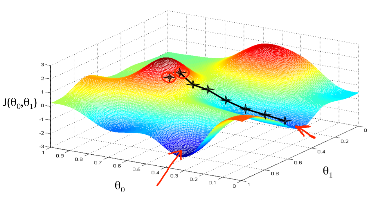
You can get stuck in local minima (if the loss is not fully convex)
If you have many model parameters, this is less likely
You always find a way down in some direction
Models with many parameters typically find good local minima
Intuition: walking downhill using only the slope you “feel” nearby

(Image by A. Karpathy)
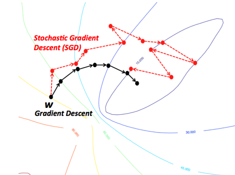
Stochastic Gradient Descent (SGD)
Compute gradients not on the entire dataset, but on a single data point at a time
Gradient descent:
Stochastic Gradient Descent:
Many smoother variants, e.g.
Minibatch SGD: compute gradient on batches of data:
Stochastic Average Gradient Descent (SAG). With randomly chosen per iteration:
Incremental gradient: with
In practice
Linear regression can be found in
sklearn.linear_model. We’ll evaluate it on the Boston Housing dataset.LinearRegressionuses closed form solution,SGDRegressorwithloss='squared_loss'uses Stochastic Gradient DescentLarge coefficients signal overfitting
Test score is much lower than training score
Source
from sklearn.model_selection import train_test_split
from sklearn.linear_model import LinearRegression

X_B, y_B = mglearn.datasets.load_extended_boston()
X_B_train, X_B_test, y_B_train, y_B_test = train_test_split(X_B, y_B, random_state=0)

lr = LinearRegression().fit(X_B_train, y_B_train)
Source
print("Weights (coefficients): {}".format(lr.coef_[0:40]))
print("Bias (intercept): {}".format(lr.intercept_))
Weights (coefficients): [ -412.711 -52.243 -131.899 -12.004 -15.511 28.716 54.704
-49.535 26.582 37.062 -11.828 -18.058 -19.525 12.203
2980.781 1500.843 114.187 -16.97 40.961 -24.264 57.616
1278.121 -2239.869 222.825 -2.182 42.996 -13.398 -19.389
-2.575 -81.013 9.66 4.914 -0.812 -7.647 33.784
-11.446 68.508 -17.375 42.813 1.14 ]
Bias (intercept): 30.934563673643545
Source
print("Training set score (R^2): {:.2f}".format(lr.score(X_B_train, y_B_train)))
print("Test set score (R^2): {:.2f}".format(lr.score(X_B_test, y_B_test)))
Training set score (R^2): 0.95
Test set score (R^2): 0.61
Ridge regression
Adds a penalty term to the least squares loss function:
Model is penalized if it uses large coefficients ()
Each feature should have as little effect on the outcome as possible
We don’t want to penalize , so we leave it out
Regularization: explicitly restrict a model to avoid overfitting.
Called L2 regularization because it uses the L2 norm:
The strength of the regularization can be controlled with the hyperparameter.
Increasing causes more regularization (or shrinkage). Default is 1.0.
Still convex. Can be optimized in different ways:
Closed form solution (a.k.a. Cholesky):
Gradient descent and variants, e.g. Stochastic Average Gradient (SAG,SAGA)
Conjugate gradient (CG): each new gradient is influenced by previous ones
Use Cholesky for smaller datasets, Gradient descent for larger ones
Ridge Regression Derivation
We want to minimize the Ridge loss function with respect to :
Expanding:
Taking the derivative with respect to :
Setting the derivative equal to zero:
In practice
from sklearn.linear_model import Ridge
lr = Ridge().fit(X_train, y_train)
Source
from sklearn.linear_model import Ridge
ridge = Ridge().fit(X_B_train, y_B_train)
print("Weights (coefficients): {}".format(ridge.coef_[0:40]))
print("Bias (intercept): {}".format(ridge.intercept_))
print("Training set score: {:.2f}".format(ridge.score(X_B_train, y_B_train)))
print("Test set score: {:.2f}".format(ridge.score(X_B_test, y_B_test)))
Weights (coefficients): [-1.414 -1.557 -1.465 -0.127 -0.079 8.332 0.255 -4.941 3.899 -1.059
-1.584 1.051 -4.012 0.334 0.004 -0.849 0.745 -1.431 -1.63 -1.405
-0.045 -1.746 -1.467 -1.332 -1.692 -0.506 2.622 -2.092 0.195 -0.275
5.113 -1.671 -0.098 0.634 -0.61 0.04 -1.277 -2.913 3.395 0.792]
Bias (intercept): 21.390525958610052
Training set score: 0.89
Test set score: 0.75
Test set score is higher and training set score lower: less overfitting!
We can plot the weight values for differents levels of regularization to explore the effect of .
Increasing regularization decreases the values of the coefficients, but never to 0.
Source
from __future__ import print_function
import ipywidgets as widgets
from ipywidgets import interact, interact_manual
from sklearn.linear_model import Ridge

@interact
def plot_ridge(alpha=(0,10.0,1)):
    r = Ridge(alpha=alpha).fit(X_B_train, y_B_train)
    fig, ax = plt.subplots(figsize=(8*fig_scale,1.5*fig_scale))
    ax.plot(r.coef_, 'o', markersize=3)
    ax.set_title("alpha {}, score {:.2f} (training score {:.2f})".format(alpha, r.score(X_B_test, y_B_test), r.score(X_B_train, y_B_train)))
    ax.set_xlabel("Coefficient index")
    ax.set_ylabel("Coefficient magnitude")
    ax.hlines(0, 0, len(r.coef_))
    ax.set_ylim(-25, 25)
    ax.set_xlim(0, 50)
Output
Source
if not interactive:
    for alpha in [0.1, 10]:
plot_ridge(alpha)When we plot the train and test scores for every value, we see a sweet spot around
Models with smaller are overfitting
Models with larger are underfitting
Source
alpha=np.logspace(-3,2,num=20)
ai = list(range(len(alpha)))
test_score=[]
train_score=[]
for a in alpha:
    r = Ridge(alpha=a).fit(X_B_train, y_B_train)
    test_score.append(r.score(X_B_test, y_B_test))
    train_score.append(r.score(X_B_train, y_B_train))
fig, ax = plt.subplots(figsize=(6*fig_scale,4*fig_scale))
ax.set_xticks(range(20))
ax.set_xticklabels(np.round(alpha,3))
ax.set_xlabel('alpha')
ax.plot(test_score, lw=2*fig_scale, label='test score')
ax.plot(train_score, lw=2*fig_scale, label='train score')
ax.legend()
plt.xticks(rotation=45);Other ways to reduce overfitting
Add more training data: with enough training data, regularization becomes less important
Ridge and ordinary least squares will have the same performance
Use fewer features: remove unimportant ones or find a low-dimensional embedding (e.g. PCA)
Fewer coefficients to learn, reduces the flexibility of the model
Scaling the data typically helps (and changes the optimal value)
Source
fig, ax = plt.subplots(figsize=(10*fig_scale,4*fig_scale))
mglearn.plots.plot_ridge_n_samples(ax)Lasso (Least Absolute Shrinkage and Selection Operator)
Adds a different penalty term to the least squares sum:
Called L1 regularization because it uses the L1 norm
Will cause many weights to be exactly 0
Same parameter to control the strength of regularization.
Will again have a ‘sweet spot’ depending on the data
No closed-form solution
Convex, but no longer strictly convex, and not differentiable
Weights can be optimized using coordinate descent
Analyze what happens to the weights:
L1 prefers coefficients to be exactly zero (sparse models)
Some features are ignored entirely: automatic feature selection
How can we explain this?
Source
from sklearn.linear_model import Lasso

@interact
def plot_lasso(alpha=(0,0.5,0.005)):
    r = Lasso(alpha=alpha).fit(X_B_train, y_B_train)
    fig, ax = plt.subplots(figsize=(8*fig_scale,1.5*fig_scale))
    ax.plot(r.coef_, 'o', markersize=6*fig_scale)
    ax.set_title("alpha {}, score {:.2f} (training score {:.2f})".format(alpha, r.score(X_B_test, y_B_test), r.score(X_B_train, y_B_train)), pad=0.5)
    ax.set_xlabel("Coefficient index", labelpad=0)
    ax.set_ylabel("Coefficient magnitude")
    ax.hlines(0, 0, len(r.coef_))
    ax.set_ylim(-25, 25);
    ax.set_xlim(0, 50);
Output
Source
if not interactive:
    for alpha in [0.00001, 0.01]:
plot_lasso(alpha)Coordinate descent
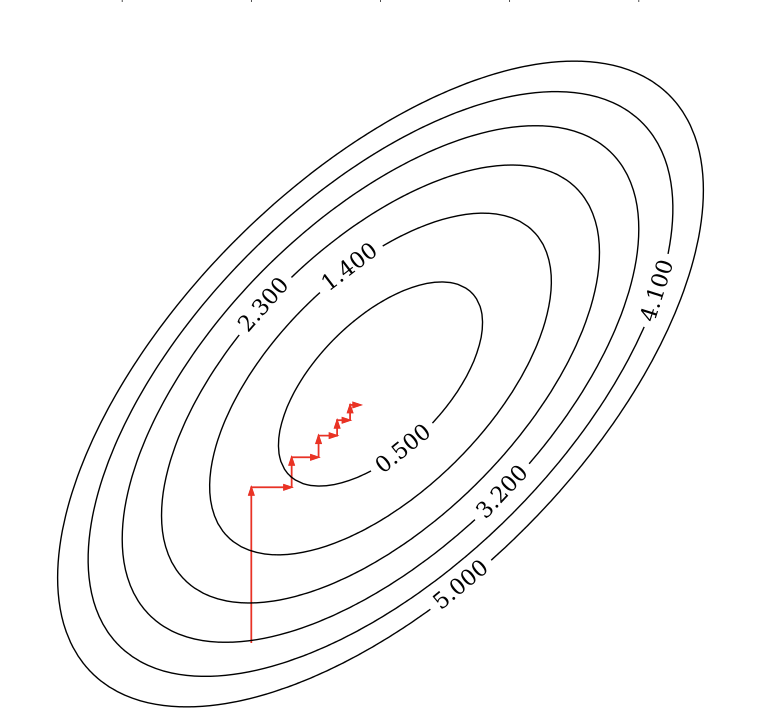
Alternative for gradient descent, supports non-differentiable convex loss functions (e.g. )
In every iteration, optimize a single coordinate (find minimum in direction of )
Continue with another coordinate, using a selection rule (e.g. round robin)
Faster iterations. No need to choose a step size (learning rate).
May converge more slowly. Can’t be parallellized.
Coordinate descent with Lasso (Further Reading)
Remember that
For one :
The L1 term is not differentiable but convex: we can compute the subgradient
Unique at points where is differentiable, a range of all possible slopes [a,b] where it is not
For , the subgradient =
Subdifferential if and are both convex
To find the optimum for Lasso , solve
In which is the part of excluding (assume for now)
can be seen as the ‘solution’: if
We found:
The Lasso solution has the form of a soft thresholding function
Small weights become 0: sparseness!
If the data is not normalized, with constant
Ridge solution: , thus
For mor information see Rashidabadi (2016)
Notebook Cell
Source
@interact
def plot_rho(alpha=(0,2.0,0.05)):
    w = np.linspace(-2,2,101)
    r = w/(1+2*alpha)
    l = [x+alpha if x <= -alpha else (x-alpha if x > alpha else 0) for x in w]
    fig, ax = plt.subplots(figsize=(6*fig_scale,3*fig_scale))
    ax.set_xlabel(r'$\rho$')
    ax.set_ylabel(r'$w^{*}$')
    ax.plot(w, w, lw=2*fig_scale, c='g', label='Ordinary Least Squares (SSE)')
    ax.plot(w, r, lw=2*fig_scale, c='b', label='Ridge with alpha={}'.format(alpha))
    ax.plot(w, l, lw=2*fig_scale, c='r', label='Lasso with alpha={}'.format(alpha))
    ax.legend()
    plt.grid()
Output
Notebook Cell
Source
if not interactive:
plot_rho(alpha=1)Interpreting L1 and L2 loss
Notebook Cell
Notebook Cell
Notebook Cell
Source
def c_fx(x):
    fX = ((x * 2 - 1)**2) # Some convex function to represent the loss
    return fX/9 # Scaling
def c_fl2(x,alpha):
    return c_fx(x) + alpha * x**2
def c_fl1(x,alpha):
    return c_fx(x) + alpha * abs(x)
def l2(x,alpha):
    return alpha * x**2
def l1(x,alpha):
    return alpha * abs(x)

@interact
def plot_losses(alpha=(0,1.0,0.05)):
    w = np.linspace(-1,1,101)
    f = [c_fx(i) for i in w]
    r = [c_fl2(i,alpha) for i in w]
    l = [c_fl1(i,alpha) for i in w]
    rp = [l2(i,alpha) for i in w]
    lp = [l1(i,alpha) for i in w]
    fig, ax = plt.subplots(figsize=(8*fig_scale,4*fig_scale))
    ax.set_xlabel('w')
    ax.set_ylabel('loss')
    ax.plot(w, rp, lw=1.5*fig_scale, ls=':', c='b', label='L2 with alpha={}'.format(alpha))
    ax.plot(w, lp, lw=1.5*fig_scale, ls=':', c='r', label='L1 with alpha={}'.format(alpha))
    ax.plot(w, f, lw=2*fig_scale, ls='-', c='k', label='Least Squares loss')
    ax.plot(w, r, lw=2*fig_scale, ls='-', c='b', label='Loss + L2 (Ridge)'.format(alpha))
    ax.plot(w, l, lw=2*fig_scale, ls='-', c='r', label='Loss + L1 (Lasso)'.format(alpha))
    opt_f = np.argmin(f)
    ax.scatter(w[opt_f], f[opt_f], c="k", s=50*fig_scale)
    opt_r = np.argmin(r)
    ax.scatter(w[opt_r], r[opt_r], c="b", s=50*fig_scale)
    opt_l = np.argmin(l)
    ax.scatter(w[opt_l], l[opt_l], c="r", s=50*fig_scale)
    ax.legend()
    box = ax.get_position()
    ax.set_position([box.x0, box.y0, box.width * 0.8, box.height])
    ax.legend(loc='center left', bbox_to_anchor=(1, 0.5))
    plt.ylim(-0.1,1)
    plt.grid()
Output
Notebook Cell
Source
if not interactive:
plot_losses(alpha=0.5)In 2D (for 2 model weights and )
The least squared loss is a 2D convex function in this space
For illustration, assume that L1 loss = L2 loss = 1
L1 loss (): every {} falls on the diamond
L2 loss (): every {} falls on the circle
For L1, the loss is minimized if or is 0 (rarely so for L2)
Source
def plot_loss_interpretation():
    line = np.linspace(-1.5, 1.5, 1001)
    xx, yy = np.meshgrid(line, line)

    l2 = xx ** 2 + yy ** 2
    l1 = np.abs(xx) + np.abs(yy)
    rho = 0.7
    elastic_net = rho * l1 + (1 - rho) * l2

    plt.figure(figsize=(5*fig_scale, 4*fig_scale))
    ax = plt.gca()

    elastic_net_contour = plt.contour(xx, yy, elastic_net, levels=[1], linewidths=2*fig_scale, colors="darkorange")
    l2_contour = plt.contour(xx, yy, l2, levels=[1], linewidths=2*fig_scale, colors="c")
    l1_contour = plt.contour(xx, yy, l1, levels=[1], linewidths=2*fig_scale, colors="navy")
    ax.set_aspect("equal")
    ax.spines['left'].set_position('center')
    ax.spines['right'].set_color('none')
    ax.spines['bottom'].set_position('center')
    ax.spines['top'].set_color('none')

    plt.clabel(elastic_net_contour, inline=1, fontsize=12*fig_scale,
               fmt={1.0: 'elastic-net'}, manual=[(-0.6, -0.6)])
    plt.clabel(l2_contour, inline=1, fontsize=12*fig_scale,
               fmt={1.0: 'L2'}, manual=[(-0.5, -0.5)])
    plt.clabel(l1_contour, inline=1, fontsize=12*fig_scale,
               fmt={1.0: 'L1'}, manual=[(-0.5, -0.5)])

    x1 = np.linspace(0.5, 1.5, 100)
    x2 = np.linspace(-1.0, 1.5, 100)
    X1, X2 = np.meshgrid(x1, x2)
    y = np.sqrt(np.square(X1/2-0.7) + np.square(X2/4-0.28))
    cp = plt.contour(X1, X2, y)
    #plt.clabel(cp, inline=1, fontsize=10)
    ax.tick_params(axis='both', pad=0)

    plt.tight_layout()
    plt.show()
plot_loss_interpretation()Comparing Ridge and LASSO for Prediction and Feature Selection
The following code trains and compares Linear Regression, Ridge (L2), and LASSO (L1) regression models. We’ll examine their predictive performance using Mean Squared Error (MSE) and observe how LASSO can be used for feature selection by shrinking some feature coefficients to zero.
Source
import numpy as np
import pandas as pd
from sklearn.linear_model import Ridge, Lasso, LinearRegression
from sklearn.metrics import mean_squared_error
from sklearn.model_selection import train_test_split
import mglearn
import warnings
from sklearn.exceptions import InconsistentVersionWarning # More specific if available, or use UserWarning

# Suppress the specific UserWarning from _openml.py
warnings.filterwarnings("ignore", category=UserWarning, module="sklearn.datasets._openml")

# Load extended Boston dataset (with polynomial features)
X_B, y_B = mglearn.datasets.load_extended_boston()
X_B_train, X_B_test, y_B_train, y_B_test = train_test_split(X_B, y_B, random_state=0)
# Train models
lr = LinearRegression().fit(X_B_train, y_B_train)
ridge = Ridge(alpha=0.2).fit(X_B_train, y_B_train)
lasso = Lasso(alpha=0.01, max_iter=5000).fit(X_B_train, y_B_train) # Increased max_iter for convergence
# Compare errors
print("Linear Regression MSE:", mean_squared_error(y_B_test, lr.predict(X_B_test)))
print("Ridge MSE:", mean_squared_error(y_B_test, ridge.predict(X_B_test)))
print("LASSO MSE:", mean_squared_error(y_B_test, lasso.predict(X_B_test)))
# Feature selection with LASSO (non-zero coefficients)
feature_names = [f"Feature {i}" for i in range(X_B.shape[1])]
lasso_coef = pd.Series(lasso.coef_, index=feature_names)
lasso_nnz = len(lasso_coef[lasso_coef != 0])
print(f"\nLASSO selected {lasso_nnz} features from total {len(lasso_coef)} features.")
Linear Regression MSE: 32.06913512158206
Ridge MSE: 18.386795859109146
LASSO MSE: 19.145582778836758

LASSO selected 33 features from total 104 features.
Elastic-Net
Adds both L1 and L2 regularization:
is the L1 ratio
With ,
With ,
sets a trade-off between L1 and L2.
Allows learning sparse models (like Lasso) while maintaining L2 regularization benefits
E.g. if 2 features are correlated, Lasso likely picks one randomly, Elastic-Net keeps both
Weights can be optimized using coordinate descent (similar to Lasso)
Sparse Optimization: Theory and Applications
Sparse optimization is a fundamental paradigm in mathematical modeling that seeks solutions with few non-zero elements, often formalized through ℓ₁-norm regularization or non-convex penalties. This framework is grounded in the Compressed Sensing (CS) theory Donoho (2006), which guarantees exact signal recovery from sub-Nyquist measurements if the signal is sparse in some basis. Key applications include:
Medical Imaging: CS enables faster MRI scans by reconstructing images from limited k-space samples (Lustig et al., 2007), as highlighted in the CUHK lecture notes on CS (p. 13).
Signal Processing: Sparse methods underpin denoising (e.g., wavelet shrinkage) and inpainting, where total variation minimization preserves edges while removing noise (Figueiredo, 2021, slides p. 8).
Machine Learning: Sparse regression (e.g., LASSO; Tibshirani, 1996) and robust PCA (Candès et al., 2011) are critical for feature selection and anomaly detection. The Ghent tutorial (p. 5) further links sparsity to deep network pruning.
Statistics: High-dimensional inference (e.g., genomics) benefits from sparsity-induced interpretability (Bühlmann & Van de Geer, 2011).
The field continues to evolve with non-convex penalties (e.g., SCAD) and greedy algorithms (OMP), balancing computational efficiency and statistical guarantees. For a unified perspective, see the cited references and tutorials.
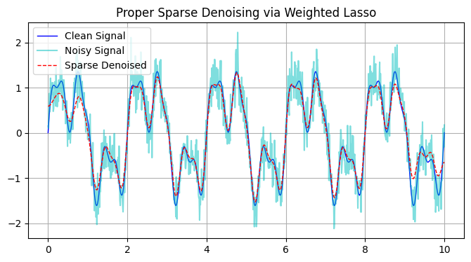
Sparse Signal Denoising via Weighted Lasso in DCT Domain
Given a noisy 1D signal:
where:
f(t)is the clean signal (sparse in frequency domain)ϵ(t)is Gaussian noise (non-sparse in any basis)
We solve the weighted Lasso problem:
Notebook Cell
Noise-Sparsity Dichotomy
Signal: Sparse in DCT domain (few dominant coefficients)
Noise: Non-sparse (energy spread across all frequencies)
Weighted ℓ₁ Magic
Preserves signal structure (low frequencies)
Aggressively truncates noise (high frequencies)
Performance Analysis
Theoretical Guarantees
Exact Recovery: Possible if:
Signal truly sparse in DCT basis
Noise level below threshold (Donoho et al., 2006)
Stability: Weighted Lasso provides better coefficient preservation than standard Lasso
Limitations
Assumes signal sparsity in chosen basis
Requires tuning for each application
Computationally heavier than simple filtering
Signal Denoising using LASSO
Source
import numpy as np
import matplotlib.pyplot as plt
from scipy.fftpack import dct, idct
from sklearn.linear_model import Lasso

# Generate clean signal with multiple frequencies
np.random.seed(42)
t = np.linspace(0, 10, 1000)
f_clean = (np.sin(2*np.pi*0.5*t) +
           0.7*np.sin(2*np.pi*1.5*t - 0.2) +
           0.3*np.sin(2*np.pi*3*t + 0.5))

# Add noise
noise = 0.3 * np.random.randn(len(t))
f_noisy = f_clean + noise

def sparse_denoise(signal, alpha=0.05):
    """Denoise using Lasso in DCT domain with proper frequency retention"""
    # DCT transform (sparse representation)
    dct_coeffs = dct(signal, norm='ortho')

    model = Lasso(alpha=alpha,
                  max_iter=10000,
                  warm_start=True,
                  selection='random')
    model.coef_ = dct_coeffs  # Initialize with DCT coeffs

    # Solve ||y - DCT^-1(x)||² + alpha * ||x||₁
    X = np.eye(len(signal))
    model.fit(X, dct_coeffs)

    # Count total number of coefficients
    total_coefs = model.coef_.shape[0]
    # Count number of non-zero coefficients (NNZ)
    nnz_count = np.count_nonzero(model.coef_)

    print(f"Total number of coefficients: {total_coefs}")
    print(f"Number of non-zero coefficients (NNZ): {nnz_count}")

    return idct(model.coef_, norm='ortho')

# Denoise with proper parameters
f_denoised = sparse_denoise(f_noisy, alpha=0.0009)

# Plot
plt.figure(figsize=(8, 4))
plt.plot(t, f_clean, 'b-', lw=1, label='Clean Signal')
plt.plot(t, f_noisy, 'c-', alpha=0.5, label='Noisy Signal')
plt.plot(t, f_denoised, 'r--', lw=1, label='Sparse Denoised')
plt.legend()
plt.title('Proper Sparse Denoising via Weighted Lasso')
plt.grid(True)
plt.show()
Total number of coefficients: 1000
Number of non-zero coefficients (NNZ): 25
Orthogonal Matching Pursuit (OMP) for Sparse Recovery
Orthogonal Matching Pursuit (OMP) is a greedy algorithm that solves the sparse approximation problem:
Problem Statement: Given a design matrix (where typically ) and observations , find the sparsest vector such that .
Key characteristics:
Iterative approach that selects one feature per iteration based on maximum correlation
Provides exact recovery guarantees under Restricted Isometry Property (RIP) conditions
Computationally efficient ( complexity) compared to -norm minimization
Widely used in compressed sensing, signal processing, and feature selection
Preserves interpretability through explicit feature selection
This method complements LASSO by offering an alternative approach to sparse recovery with distinct theoretical guarantees and computational trade-offs.
While LASSO solves the -regularized problem:
OMP provides a greedy alternative for sparse approximation, solving:
OMP algorithm
Given:
Design matrix
Response vector
Target sparsity level
At each iteration:
Select most correlated feature: , where is the current residual and is the active feature set.
Update support:
Solve least squares:
Update residual:
Termination: After iterations or when
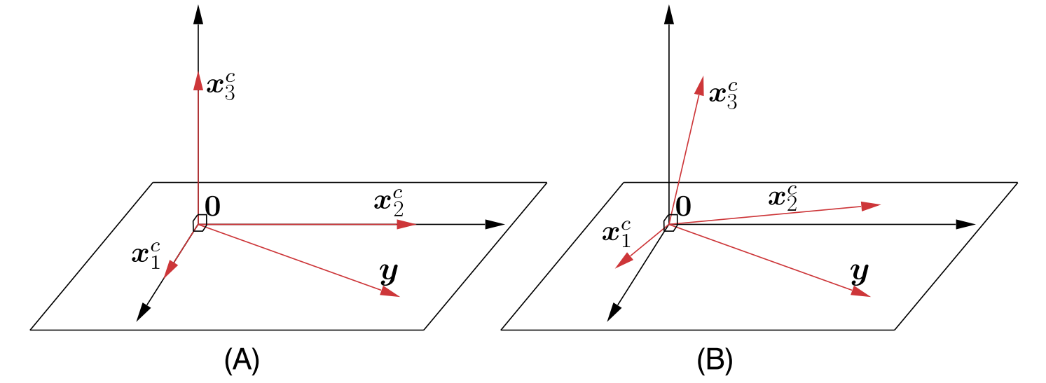
Figure 10.2 of Theodoridis (2020):
(A) In the case of an orthogonal matrix, the observations vector y will be orthogonal to any inactive column, here, . (B) In the more general case, it is expected to “lean” closer (form smaller angles) to the active than to the inactive columns.
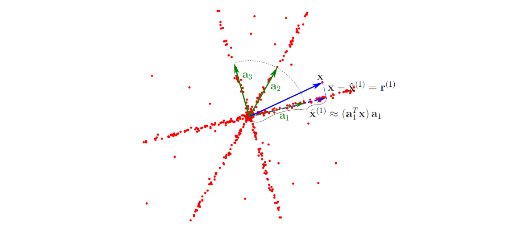
Figure 2.3 of Bakhshali (2018)
Comparison with LASSO
| Property | OMP | LASSO |
|---|---|---|
| Objective | constraint | regularization |
| Solution | Greedy approximation | Convex optimization |
| Computational | Faster for small | Slower but more stable |
| Theoretical | Exact recovery possible | Consistent estimation |
For further information see Asaran (2016).
Practice
import numpy as np
from numpy.linalg import pinv

def omp(X, y, k, tol=1e-6):
    """
    Orthogonal Matching Pursuit

    Parameters
    ----------
    X : ndarray, shape (n_samples, n_features)
        Design matrix
    y : ndarray, shape (n_samples,)
        Target vector
    k : int
        Sparsity level (number of non-zero coefficients)
    tol : float
        Residual tolerance for early stopping

    Returns
    -------
    w : ndarray, shape (n_features,)
        Sparse coefficient vector
    """
    n, p = X.shape
    w = np.zeros(p)
    residual = y.copy()
    active = []

    for _ in range(k):
        # Find most correlated feature
        correlations = np.abs(X.T @ residual)
        correlations[active] = -np.inf  # exclude selected
        new_idx = np.argmax(correlations)
        active.append(new_idx)

        # Solve least squares on active set
        X_active = X[:, active]
        w_active = pinv(X_active) @ y

        # Update residual
        residual = y - X_active @ w_active

        # Early stopping if residual is small
        if np.linalg.norm(residual) < tol:
            break

    # Convert to full coefficient vector
    w_sparse = np.zeros(p)
    w_sparse[active] = w_active
    return w_sparse
Source
import numpy as np
import matplotlib.pyplot as plt
from sklearn.linear_model import Lasso

# Generate synthetic data
np.random.seed(42)
n, p = 100, 200
X = np.random.randn(n, p)
w_true = np.zeros(p)
w_true[[5, 45, 100]] = [1.5, -0.8, 1.2]
y = X @ w_true + 0.1 * np.random.randn(n)

# Split into train/test (80/20)
split_idx = int(0.8 * n)
X_train, X_test = X[:split_idx], X[split_idx:]
y_train, y_test = y[:split_idx], y[split_idx:]

# --- Run OMP ---
w_omp = omp(X_train, y_train, k=3)

# --- Run LASSO ---
lasso = Lasso(alpha=0.1).fit(X_train, y_train)
w_lasso = lasso.coef_

# --- Evaluation Metrics ---
# Print ground truth for reference
true_nnz = w_true[w_true != 0]
print("\nGround Truth Non-zero Coefficients:", ", ".join([f"{val:.2f}" for val in true_nnz]))

print("\nPerformance Comparison:")
print(f"{'Method':<10} {'Test MSE':<12} {'Support Error':<15} {'ℓ2 Error':<10} {'Non-zero Coefficients':<30}")
print("-"*75)

for name, w in [('OMP', w_omp), ('LASSO', w_lasso)]:
    test_mse = np.mean((X_test @ w - y_test)**2)
    support_error = np.sum((w != 0) != (w_true != 0))
    l2_error = np.linalg.norm(w - w_true)
    nnz_values = w[w != 0]

    # Format NNZ values with 2 decimal places
    nnz_str = ", ".join([f"{val:.2f}" for val in nnz_values[:5]])  # Show first 5
    if len(nnz_values) > 5:
        nnz_str += ", ..."

    print(f"{name:<10} {test_mse:.4e}    {support_error:<15} {l2_error:<10.4f} [{nnz_str}]")
Ground Truth Non-zero Coefficients: 1.50, -0.80, 1.20

Performance Comparison:
Method     Test MSE     Support Error   ℓ2 Error   Non-zero Coefficients
---------------------------------------------------------------------------
OMP        1.6293e-02    0               0.0296     [1.51, -0.80, 1.17]
LASSO      5.5046e-02    0               0.2214     [1.39, -0.68, 1.05]
Notebook Cell
# --- Coefficient Visualization ---
plt.figure(figsize=(4, 8*fig_scale))

# OMP Plot
plt.subplot(2, 1, 1)
plt.stem(w_omp, markerfmt='ro', basefmt=" ")
plt.title(f"OMP Coefficients\n(Test MSE: {np.mean((X_test @ w_omp - y_test)**2):.2e})")
plt.xlabel("Feature Index")
plt.ylabel("Coefficient Value")
plt.axhline(0, color='k', linestyle='--', alpha=0.3)
plt.xlim(0, p)

# LASSO Plot
plt.subplot(2, 1, 2)
plt.stem(w_lasso, markerfmt='bo', basefmt=" ")
plt.title(f"LASSO Coefficients (α=0.1)\n(Test MSE: {np.mean((X_test @ w_lasso - y_test)**2):.2e})")
plt.xlabel("Feature Index")
plt.ylabel("Coefficient Value")
plt.axhline(0, color='k', linestyle='--', alpha=0.3)
plt.xlim(0, p)

plt.tight_layout()
plt.show()A Simple Example
Source
import numpy as np
from numpy.linalg import pinv

def omp_with_steps(X, y, k, tol=1e-6):
    """
    Orthogonal Matching Pursuit with step-by-step printing

    Parameters
    ----------
    X : ndarray, shape (n_samples, n_features)
        Design matrix (should be shape (3, 5) for this example)
    y : ndarray, shape (n_samples,)
        Target vector (should be shape (3,) for this example)
    k : int
        Sparsity level (number of non-zero coefficients)
    tol : float
        Residual tolerance for early stopping

    Returns
    -------
    w : ndarray, shape (n_features,)
        Sparse coefficient vector
    """
    n, p = X.shape
    w = np.zeros(p)
    residual = y.copy()
    active = []

    print("=== Orthogonal Matching Pursuit ===")
    print(f"Target vector y: {y}")
    print(f"Initial residual norm: {np.linalg.norm(residual):.4f}\n")

    for iteration in range(k):
        # Find most correlated feature
        correlations = np.abs(X.T @ residual)

        # Exclude already selected indices (avoid OverflowError)
        if active:
            correlations[active] = -np.inf

        new_idx = np.argmax(correlations)
        active.append(new_idx)

        # Solve least squares on active set
        X_active = X[:, active]
        w_active = pinv(X_active) @ y

        # Update residual
        residual = y - X_active @ w_active

        # Print step information
        print(f"Iteration {iteration + 1}:")
        print(f"  Selected index: {new_idx}")
        print(f"  Active set: {active}")
        print(f"  Coefficients: {w_active}")
        print(f"  Residual norm: {np.linalg.norm(residual):.4f}\n")
        print(f"  {X_active.shape}, {pinv(X_active).shape}, {w_active.shape}\n")

        # Early stopping if residual is small
        if np.linalg.norm(residual) < tol:
            print(f"Stopping early: residual norm {np.linalg.norm(residual):.4f} < tolerance {tol}")
            break

    # Convert to full coefficient vector
    w_sparse = np.zeros(p)
    w_sparse[active] = w_active
    print("\n=== Final Result ===")
    print(f"Non-zero coefficients at indices: {np.nonzero(w_sparse)[0]}")
    print(f"Coefficient values: {w_sparse[w_sparse != 0]}")
    return w_sparse

# Example usage
if __name__ == "__main__":
    # Correct initialization: A should be (3, 5) for Ax=b where b is (3,)
    A = np.array([
        [1, 0, 0, 1],  # x-components of basis vectors
        [0, 1, 0, 1], # y-components of basis vectors
        [0, 0, 1, 0]   # z-components of basis vectors
    ])  # Shape (3, 5)

    # Target vector in xy-plane
    b = np.array([2, 3, 0])

    print("Dictionary matrix A (shape {}):".format(A.shape))
    print(A)
    print("\nTarget vector b:", b)
    print("\nRunning OMP with k=2...\n")

    # Run OMP with step printing
    w_sparse = omp_with_steps(A, b, k=2)

    # Verify reconstruction
    reconstruction = A @ w_sparse
    print("\nReconstruction:", reconstruction)
    print("Target:", b)
    print("Reconstruction error:", np.linalg.norm(reconstruction - b))
Dictionary matrix A (shape (3, 4)):
[[1 0 0 1]
[0 1 0 1]
[0 0 1 0]]
Target vector b: [2 3 0]
Running OMP with k=2...
=== Orthogonal Matching Pursuit ===
Target vector y: [2 3 0]
Initial residual norm: 3.6056
Iteration 1:
Selected index: 3
Active set: [np.int64(3)]
Coefficients: [2.5]
Residual norm: 0.7071
(3, 1), (1, 3), (1,)
Iteration 2:
Selected index: 1
Active set: [np.int64(3), np.int64(1)]
Coefficients: [2. 1.]
Residual norm: 0.0000
(3, 2), (2, 3), (2,)
Stopping early: residual norm 0.0000 < tolerance 1e-06
=== Final Result ===
Non-zero coefficients at indices: [1 3]
Coefficient values: [1. 2.]
Reconstruction: [2. 3. 0.]
Target: [2 3 0]
Reconstruction error: 6.280369834735101e-16
When to Use OMP
Exactly sparse signals – OMP is ideal when the underlying signal truly has only a few non-zero coefficients, making it a strong choice for enforcing strict sparsity.
Small-scale problems – Works efficiently when the number of non-zero elements is much smaller than the total features (i.e., ), preventing unnecessary computational overhead.
Interpretable solutions – Since OMP selects features iteratively, the stepwise approach makes it easier to analyze which features contribute to the model, often simpler than interpreting LASSO’s continuous shrinkage.
Dictionary learning – Frequently used in sparse coding applications, where signals are represented as a sparse combination of dictionary elements, making it valuable for feature selection in compressed sensing.
Similarities and Differences in Solving in Regression and Sparse Representation
Similarities
Core Equation: Both domains solve the linear system .
Matrix-Vector Structure:
is a matrix, is a vector of unknowns, and is a vector of observations/targets.
Optimization Goal: Both aim to find such that approximates , often with a minimization objective (e.g., least squares or sparsity constraints).
Differences in Specification of 
| Aspect | Regression | Sparse Representation |
|---|---|---|
| Role of | Design matrix: Rows = samples, columns = features. - Each row is a data sample (e.g., patient measurements). - Each column is a feature (e.g., age, blood pressure). | Dictionary matrix: Columns = atoms/basis vectors. - Each column is a pre-defined basis (e.g., wavelets, image patches). - Typically overcomplete (more columns than rows). |
| Role of | Coefficient vector: Represents weights for features. - = weight for the -th feature. - Usually dense (all entries non-zero). | Sparse coefficient vector: Represents activations of atoms. - = activation of the -th atom. - Must be sparse (most entries zero). |
| Role of | Target vector: Observed responses for samples. - = target value for the -th sample (e.g., house price). | Signal vector: Input signal to be represented. - = value at the -th dimension (e.g., pixel intensity). |
| Problem Goal | Model relationships: Predict from features in . | Compress/denoise signals: Represent as a sparse combination of atoms in . |
| Solution Method | Least squares: Minimize . - Closed-form: . | Sparsity-constrained optimization: Minimize (LASSO) or (non-convex). |
| Key Assumption | Features are independent/linearly related. | Signal can be represented by few atoms from . |
| Example Use Case | Predicting house prices from features (size, location). | Denoising an image using a dictionary of edges/textures. |
Key Differences Explained
Structure of :
Regression: is tall/square (rows ≥ columns). Rows = samples, columns = features.
Example: 100 patients (rows) × 5 features (columns).Sparse Representation: is fat (columns > rows). Columns = atoms, rows = signal dimensions.
Example: 1000 pixels (rows) × 5000 atoms (columns).
Sparsity of :
Regression: is dense (all entries non-zero). Every feature contributes to predictions.
Sparse Representation: must be sparse (most entries zero). Only a few atoms are activated.
Interpretation:
Regression: quantifies feature importance (e.g., “size” has weight 0.8).
Sparse Representation: identifies active atoms (e.g., “edge #42” is activated for a line in an image).
Optimization:
Regression: Unconstrained least squares (closed-form or iterative solvers).
Sparse Representation: Constrained optimization (L1/L0 regularization) to enforce sparsity (e.g., LASSO, OMP).
Example: House Price Prediction (Regression)
: 100 houses (rows) × 3 features: [size, bedrooms, age].
: House prices (e.g., [300k, 450k, ...]).
: Weights (e.g., [size: 0.2, bedrooms: 0.1, age: -0.05]).
Solution: (dense).
Example: Image Denoising (Sparse Representation)
: Dictionary of 10,000 image patches (atoms).
: Noisy 50×50 image vectorized (2500 rows).
: Sparse vector activating 20 atoms (e.g., only 20 non-zero entries).
Solution: Minimize (sparse).
Summary
Regression: = samples × features, = dense weights, = targets. Focus on prediction.
Sparse Representation: = signal × atoms, = sparse activations, = signal. Focus on compression/denoising.
Shared Core: Both solve , but with different constraints on and interpretations of .
Connection Between Sparse Learning and Functional Analysis (Further Reading)
Sparse recovery techniques like OMP and LASSO are deeply rooted in functional analysis, which explains why terms like Hilbert spaces and Banach spaces frequently appear in machine learning research. These mathematical frameworks provide the theoretical foundation for understanding sparsity-inducing methods.
Hilbert Spaces and Orthogonal Projections
Hilbert spaces (complete inner product spaces) are essential for analyzing orthogonal projections and basis expansions. For example:
OMP iteratively projects the residual onto the span of selected basis vectors, leveraging the orthogonality principle to minimize error at each step.
The inner product structure of Hilbert spaces enables efficient computation of correlations between residuals and dictionary atoms (columns of ).
Banach Spaces and -Regularization
LASSO operates in the context of Banach spaces (complete normed vector spaces) due to its reliance on the -norm:
The -norm’s non-smoothness at the origin induces sparsity, a property studied in Banach space geometry.
Unlike Hilbert spaces, Banach spaces generalize optimization techniques to non-Euclidean settings, crucial for sparse regularization.
Fourier, Wavelet, and Other Representations
Sparse learning often exploits transform domains (e.g., Fourier, wavelet, or learned dictionaries) where signals admit concise representations: - These domains provide structured bases where only a few coefficients are significant. - The connection to functional analysis arises because such bases typically form frames or Riesz bases in Hilbert spaces, ensuring stable sparse approximations.
From Fixed Bases to Learned Representations
Classical Sparse Coding:
Relies on predefined bases (e.g., Fourier, wavelets) where signals admit sparse representations.
These bases often form frames or Riesz bases in Hilbert spaces, ensuring stable approximations.
Convolutional Neural Networks (CNNs):
Learn adaptive bases/filters from data, implicitly constructing sparse-like representations through:
Local connectivity: Filters act as localized basis functions.
Activation sparsity: ReLU promotes de facto sparsity in feature maps.
While CNNs lack explicit / constraints, their hierarchical structure approximates multi-scale sparse decompositions, akin to wavelet analysis but data-driven.
The Evolving Role of Sparse Methods
While deep learning has reduced reliance on handcrafted sparse models in some domains, sparse methods remain relevant because:
Interpretability:
OMP/LASSO yield explicit basis selections, whereas CNNs operate as black boxes.
Critical in fields like medicine or physics where model transparency is required.
Data-Efficiency:
Sparse methods often outperform DL in low-data regimes (e.g., medical imaging with small datasets).
Theoretical Guarantees:
Compressed sensing (OMP) and convex optimization (LASSO) provide recovery guarantees under precise conditions, unlike empirical DL results.
Hybrid Approaches:
Modern architectures (e.g., ISTA-Net, Learned Iterative Shrinkage) blend sparse priors with deep learning, showing that sparsity remains a useful inductive bias.
Sparse learning and deep learning are complementary:
CNNs dominate when data is abundant and interpretability is secondary.
OMP/LASSO persist in scenarios requiring rigor, efficiency, or transparency.
Functional analysis bridges these paradigms, providing tools to analyze both fixed and learned representations.
MRI reconstruction (Further Reading)
MRI reconstruction can be formulated as an inverse problem where the goal is to recover the original image from under-sampled k-space measurements . This is achieved using sparse optimization techniques.
A common formulation for MRI reconstruction is:
where:
represents the MRI image to be reconstructed.
is the under-sampled Fourier operator, mapping the image to k-space.
is the acquired k-space data (limited measurements).
is the sparsifying transform (e.g., wavelet or total variation).
represents the sparsity constraint, often chosen as (similar to LASSO) or (similar to OMP).
controls the balance between data fidelity and sparsity enforcement.
By leveraging sparsity, MRI reconstruction enables faster scans with fewer measurements while preserving essential anatomical details.
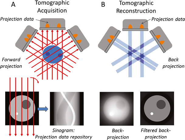
Source: Iterative reconstruction: how it works, how to apply it
PyTomography
PyTomography is an open-source Python library designed for medical image reconstruction, particularly in SPECT (Single-Photon Emission Computed Tomography) and PET (Positron Emission Tomography) imaging. Developed to address the challenges of quantitative tomographic reconstruction, PyTomography provides a flexible, modular framework for implementing advanced reconstruction algorithms, including attenuation correction, scatter correction, and resolution modeling.
Key Features
✅ Open-source & community-driven (GitHub)
✅ Supports multiple reconstruction techniques (OSEM, MLEM, deep learning-based methods)
✅ Integrates with GPU acceleration for faster computations
✅ Well-documented with tutorials and API references (ReadTheDocs)
✅ Validated in peer-reviewed research (Scientific Reports, 2024)
Why Use PyTomography?
PyTomography bridges the gap between research and clinical applications by offering:
Reproducible reconstruction workflows
Customizable forward and backward projection models
Seamless integration with Python’s scientific computing stack (NumPy, PyTorch)
Whether for academic research, algorithm development, or clinical prototyping, PyTomography provides a powerful, accessible toolkit for next-generation medical imaging reconstruction.
PySAP
The Python Sparse data Analysis Package (PySAP) was developed as part of COSMIC, a multi-disciplinary collaboration between NeuroSpin, experts in biomedical imaging, and CosmoStat, experts in astrophysical image processing. PySAP is designed to provide state-of-the-art signal processing tools for various imaging domains, including:
Astronomy
Electron Tomography
Magnetic Resonance Imaging (MRI)
One of PySAP’s core contributions lies in sparse optimization, a powerful technique widely used for reconstructing images from incomplete or noisy data. The package implements advanced compressed sensing algorithmsTheodoridis (2020), allowing efficient image restoration while preserving essential features.
In medical imaging, PySAP plays a crucial role in MRI reconstruction by leveraging sparsity-based approaches to improve scan efficiency. It enables:
Reduced scanning time while maintaining image quality
Improved reconstruction of under-sampled k-space data
Integration of machine learning techniques for further enhancement
The first release of PySAP was presented in Farrens et al. Gueddari et al. (2020) and continues to evolve as a robust tool for sparse signal processing.
For further exploration, visit the PySAP GitHub repository.
In our deep learning course, we will encounter additional examples of minimizing , including applications like image deblurring and super-resolution.
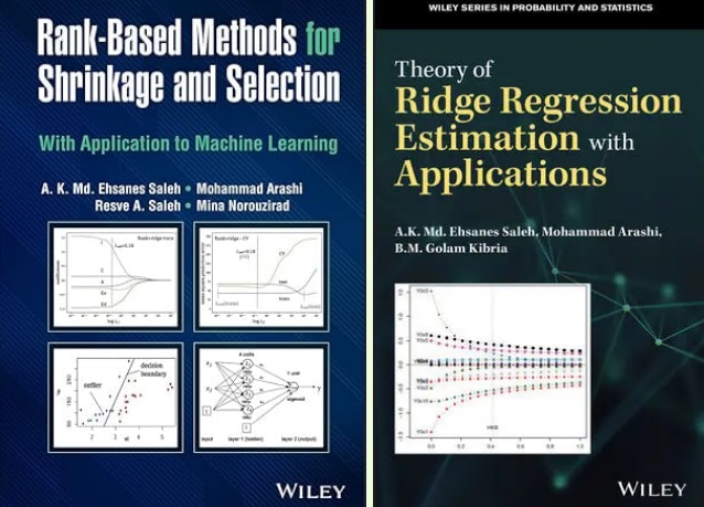
For valuable references on Ridge and Shrinkage methods, consider consulting Prof. Arashi’s books Saleh et al. (2019)Saleh et al. (2022).
Linear models for Classification
Aims to find a hyperplane that separates the examples of each class.
For binary classification (2 classes), we aim to fit the following function:
When , predict class -1, otherwise predict class +1
Source
from sklearn.linear_model import LogisticRegression
from sklearn.svm import LinearSVC

Xf, yf = mglearn.datasets.make_forge()
fig, ax = plt.subplots(figsize=(6*fig_scale,4*fig_scale))
clf = LogisticRegression().fit(Xf, yf)
mglearn.tools.plot_2d_separator(clf, Xf,
                                ax=ax, alpha=.7, cm=mglearn.cm2)
mglearn.discrete_scatter(Xf[:, 0], Xf[:, 1], yf, ax=ax, s=10*fig_scale)
ax.set_title("Logistic Regression")
ax.set_xlabel("Feature 1")
ax.set_ylabel("Feature 2")
ax.legend(['Class -1','Class 1']);There are many algorithms for linear classification, differing in loss function, regularization techniques, and optimization method
Most common techniques:
Convert target classes {neg,pos} to {0,1} and treat as a regression task
Logistic regression (Log loss)
Ridge Classification (Least Squares + L2 loss)
Find hyperplane that maximizes the margin between classes
Linear Support Vector Machines (Hinge loss)
Neural networks without activation functions
Perceptron (Perceptron loss)
SGDClassifier: can act like any of these by choosing loss function
Hinge, Log, Modified_huber, Squared_hinge, Perceptron
Logistic regression
Aims to predict the probability that a point belongs to the positive class
Converts target values {negative (blue), positive (red)} to {0,1}
Fits a logistic (or sigmoid or S curve) function through these points
Maps (-Inf,Inf) to a probability [0,1]
E.g. in 1D:
Source
def sigmoid(x,w1,w0):
    return 1 / (1 + np.exp(-(x*w1+w0)))

@interact
def plot_logreg(w0=(-10.0,5.0,1),w1=(-1.0,3.0,0.3)):
    fig, ax = plt.subplots(figsize=(8*fig_scale,3*fig_scale))
    red = [Xf[i, 1] for i in range(len(yf)) if yf[i]==1]
    blue = [Xf[i, 1] for i in range(len(yf)) if yf[i]==0]
    ax.scatter(red, [1]*len(red), c='r', label='Positive class')
    ax.scatter(blue, [0]*len(blue), c='b', label='Negative class')
    x = np.linspace(min(-1, -w0/w1),max(6, -w0/w1))
    ax.plot(x,sigmoid(x,w1,w0),lw=2*fig_scale,c='g', label='logistic(x*w1+w0)'.format(np.round(w0,2),np.round(w1,2)))
    ax.axvline(x=(-w0/w1), ymin=0, ymax=1, label='Decision boundary')
    ax.plot(x,x*w1+w0,lw=2*fig_scale,c='k',linestyle=':', label='y=x*w1+w0')
    ax.set_xlabel("Feature")
    ax.set_ylabel("y")
    ax.set_ylim(-0.05,1.05)
    ax.legend(loc='center left', bbox_to_anchor=(1, 0.5))
    box = ax.get_position()
    ax.set_position([box.x0, box.y0, box.width * 0.8, box.height]);
Output
Source
if not interactive:
    # fitted solution
    clf2 = LogisticRegression(C=100).fit(Xf[:, 1].reshape(-1, 1), yf)
    w0 = clf2.intercept_
    w1 = clf2.coef_[0][0]
plot_logreg(w0=w0,w1=w1)Fitted solution to our 2D example:
To get a binary prediction, choose a probability threshold (e.g. 0.5)
Source
lr_clf = LogisticRegression(C=100).fit(Xf, yf)

def sigmoid2d(x1,x2,w0,w1,w2):
    return 1 / (1 + np.exp(-(x2*w2+x1*w1+w0)))

@interact
def plot_logistic_fit(rotation=(0,360,10)):
    w0 = lr_clf.intercept_
    w1 = lr_clf.coef_[0][0]
    w2 = lr_clf.coef_[0][1]

    # plot surface of f
    fig = plt.figure(figsize=(7*fig_scale,5*fig_scale))
    ax = plt.axes(projection="3d")
    x0 = np.linspace(8, 16, 30)
    x1 = np.linspace(-1, 6, 30)
    X0, X1 = np.meshgrid(x0, x1)

    # Surface
    ax.plot_surface(X0, X1, sigmoid2d(X0, X1, w0, w1, w2), rstride=1, cstride=1,
                    cmap='bwr', edgecolor='none',alpha=0.5,label='sigmoid')
    # Points
    c=['b','r']
    ax.scatter3D(Xf[:, 0], Xf[:, 1], yf, c=[c[i] for i in yf], s=10*fig_scale)

    # Decision boundary
    # x2 = -(x1*w1 + w0)/w2
    ax.plot3D(x0,-(x0*w1 + w0)/w2,[0.5]*len(x0), lw=1*fig_scale, c='k', linestyle=':')
    z = np.linspace(0, 1, 31)
    XZ, Z = np.meshgrid(x0, z)
    YZ = -(XZ*w1 + w0)/w2
    ax.plot_wireframe(XZ, YZ, Z, rstride=5, lw=1*fig_scale, cstride=5, alpha=0.3, color='k',label='decision boundary')
    ax.tick_params(axis='both', width=0, labelsize=10*fig_scale, pad=-4)

    ax.set_xlabel('x0', labelpad=-6)
    ax.set_ylabel('x1', labelpad=-6)
    ax.get_zaxis().set_ticks([])
    ax.view_init(30, rotation) # Use this to rotate the figure
    plt.tight_layout()
    #plt.legend() # Doesn't work yet, bug in matplotlib
plt.show()Source
if not interactive:
plot_logistic_fit(rotation=150)Loss function: Cross-entropy (Further Reading)
Models that return class probabilities can use cross-entropy loss
Also known as log loss, logistic loss, or maximum likelihood
Based on true probabilities (0 or 1) and predicted probabilities over instances and classes
Binary case (C=2):
Penalty (or surprise) grows exponentially as difference between and increases
Often used together with L2 (or L1) loss:
We will see this loss function in Deep Learning Course
Notebook Cell
Source
def cross_entropy(yHat, y):
    if y == 1:
        return -np.log(yHat)
    else:
        return -np.log(1 - yHat)

fig, ax = plt.subplots(figsize=(6*fig_scale,2*fig_scale))
x = np.linspace(0,1,100)

ax.plot(x,cross_entropy(x, 1),lw=2*fig_scale,c='b',label='true label = 1', linestyle='-')
ax.plot(x,cross_entropy(x, 0),lw=2*fig_scale,c='r',label='true label = 0', linestyle='-')
ax.set_xlabel(r"Predicted probability $\hat{y}$")
ax.set_ylabel("Log loss")
plt.grid()
plt.legend();Optimization methods (solvers) for cross-entropy loss
Gradient descent (only supports L2 regularization)
Log loss is differentiable, so we can use (stochastic) gradient descent
Variants thereof, e.g. Stochastic Average Gradient (SAG, SAGA)
Coordinate descent (supports both L1 and L2 regularization)
Faster iteration, but may converge more slowly, has issues with saddlepoints
Called
liblinearin sklearn. Can’t run in parallel.
Newton-Rhapson or Newton Conjugate Gradient (only L2):
Uses the Hessian :
Slow for large datasets. Works well if solution space is (near) convex
Quasi-Newton methods (only L2)
Approximate, faster to compute
E.g. Limited-memory Broyden–Fletcher–Goldfarb–Shanno (
lbfgs)Default in sklearn for Logistic Regression
For further information about conjugate gradients, see Nemati (2018)
You will see many of these solvers in Optimization course taught by Dr. Ghanbari.
In practice
Logistic regression can also be found in
sklearn.linear_model.Chyperparameter is the inverse regularization strength:penalty: type of regularization: L1, L2 (default), Elastic-Net, or Nonesolver: newton-cg, lbfgs (default), liblinear, sag, saga
Increasing C: less regularization, tries to overfit individual points
from sklearn.linear_model import LogisticRegression
lr = LogisticRegression(C=1).fit(X_train, y_train)
Source
from sklearn.linear_model import LogisticRegression

@interact
def plot_lr(C_log=(-3,4,0.1)):
    # Still using artificial data
    fig, ax = plt.subplots(figsize=(6*fig_scale,3*fig_scale))
    mglearn.discrete_scatter(Xf[:, 0], Xf[:, 1], yf, ax=ax, s=10*fig_scale)
    lr = LogisticRegression(C=10**C_log).fit(Xf, yf)
    w = lr.coef_[0]
    xx = np.linspace(7, 13)
    yy = (-w[0] * xx - lr.intercept_[0]) / w[1]
    ax.plot(xx, yy, c='k')
    ax.set_xticks(())
    ax.set_yticks(())
    ax.set_title("C = {:.3f}, w1={:.3f}, w2={:.3f}".format(10**C_log,w[0],w[1]))
    ax.legend(loc="best");
Output
Source
if not interactive:
    plot_lr(C_log=(0))
plot_lr(C_log=(4))Analyze behavior on the breast cancer dataset
Underfitting if C is too small, some overfitting if C is too large
We use cross-validation because the dataset is small
Source
from sklearn.datasets import fetch_openml
from sklearn.model_selection import cross_validate

spam_data = fetch_openml(name="qsar-biodeg", as_frame=True)
X_C, y_C = spam_data.data, spam_data.target

C=np.logspace(-3,6,num=19)
test_score=[]
train_score=[]
for c in C:
    lr = LogisticRegression(C=c)
    scores = cross_validate(lr,X_C,y_C,cv=10, return_train_score=True)
    test_score.append(np.mean(scores['test_score']))
    train_score.append(np.mean(scores['train_score']))
fig, ax = plt.subplots(figsize=(6*fig_scale,4*fig_scale))
ax.set_xticks(range(19))
ax.set_xticklabels(np.round(C,3))
ax.set_xlabel('C')
ax.plot(test_score, lw=2*fig_scale, label='test score')
ax.plot(train_score, lw=2*fig_scale, label='train score')
ax.legend()
plt.xticks(rotation=45);Again, choose between L1 or L2 regularization (or elastic-net)
Small C overfits, L1 leads to sparse models
Source
X_C_train, X_C_test, y_C_train, y_C_test = train_test_split(X_C, y_C, random_state=0)

@interact
def plot_logreg(C=(0.01,1000.0,0.1), penalty=['l1','l2']):
    r = LogisticRegression(C=C, penalty=penalty, solver='liblinear').fit(X_C_train, y_C_train)
    fig, ax = plt.subplots(figsize=(8*fig_scale,1.9*fig_scale))
    ax.plot(r.coef_.T, 'o', markersize=6*fig_scale)
    ax.set_title("C: {:.3f}, penalty: {}, score {:.2f} (training score {:.2f})".format(C, penalty, r.score(X_C_test, y_C_test), r.score(X_C_train, y_C_train)),pad=0)
    ax.set_xlabel("Coefficient index", labelpad=0)
    ax.set_ylabel("Coeff. magnitude", labelpad=0, fontsize=10*fig_scale)
    ax.tick_params(axis='both', pad=0)
    ax.hlines(0, 40, len(r.coef_)-1)
    ax.set_ylim(-10, 10)
    ax.set_xlim(0, 40);
    plt.tight_layout();
Output
Source
if not interactive:
    plot_logreg(0.001, 'l2')
    plot_logreg(100, 'l2')
plot_logreg(100, 'l1')Note: Data scaling helps convergence, minimizes differences between solvers
from sklearn.linear_model import LogisticRegression
from sklearn.preprocessing import StandardScaler
from sklearn.datasets import make_classification

# Generate data with unscaled features
X, y = make_classification(n_features=2, n_redundant=0, random_state=42)
X[:, 1] *= 1000  # Artificially scale one feature

# Solvers to compare
solvers = ['newton-cg', 'lbfgs', 'liblinear', 'sag', 'saga']

# Without scaling
for solver in solvers:
    model = LogisticRegression(solver=solver, max_iter=1000)
    model.fit(X, y)
    print(f"{solver:10} → Iterations: {model.n_iter_[0]} (unscaled)")

# With scaling
scaler = StandardScaler()
X_scaled = scaler.fit_transform(X)
for solver in solvers:
    model = LogisticRegression(solver=solver, max_iter=1000)
    model.fit(X_scaled, y)
    print(f"{solver:10} → Iterations: {model.n_iter_[0]} (scaled)")
newton-cg → Iterations: 19 (unscaled)
lbfgs → Iterations: 43 (unscaled)
liblinear → Iterations: 14 (unscaled)
sag → Iterations: 1000 (unscaled)
saga → Iterations: 1000 (unscaled)
newton-cg → Iterations: 5 (scaled)
lbfgs → Iterations: 7 (scaled)
liblinear → Iterations: 5 (scaled)
sag → Iterations: 21 (scaled)
saga → Iterations: 12 (scaled)
Ridge Classification
Instead of log loss, we can also use ridge loss:
In this case, target values {negative, positive} are converted to {-1,1}
Can be solved similarly to Ridge regression:
Closed form solution (a.k.a. Cholesky)
Gradient descent and variants
E.g. Conjugate Gradient (CG) or Stochastic Average Gradient (SAG,SAGA)
Use Cholesky for smaller datasets, Gradient descent for larger ones
Linear Models for multiclass classification
one-vs-rest (aka one-vs-all)
Learn a binary model for each class vs. all other classes
Create as many binary models as there are classes
Source
from sklearn.datasets import make_blobs

X, y = make_blobs(random_state=42)
linear_svm = LinearSVC().fit(X, y)

plt.rcParams["figure.figsize"] = (7*fig_scale,5*fig_scale)
mglearn.discrete_scatter(X[:, 0], X[:, 1], y, s=10*fig_scale)
line = np.linspace(-15, 15)
for coef, intercept, color in zip(linear_svm.coef_, linear_svm.intercept_,
                                  mglearn.cm3.colors):
    plt.plot(line, -(line * coef[0] + intercept) / coef[1], c=color, lw=2*fig_scale)
plt.ylim(-10, 15)
plt.xlim(-10, 8)
plt.gca().set_aspect('equal')
plt.xlabel("Feature 0")
plt.ylabel("Feature 1")
plt.legend(['Class 0', 'Class 1', 'Class 2', 'Line class 0', 'Line class 1',
'Line class 2'], loc=(1.01, 0.3))Every binary classifiers makes a prediction, the one with the highest score (>0) wins
Source
mglearn.plots.plot_2d_classification(linear_svm, X, fill=True, alpha=0.3)
mglearn.discrete_scatter(X[:, 0], X[:, 1], y, s=10*fig_scale)
line = np.linspace(-15, 15)
for coef, intercept, color in zip(linear_svm.coef_, linear_svm.intercept_,
                                  mglearn.cm3.colors):
    plt.plot(line, -(line * coef[0] + intercept) / coef[1], c=color, lw=2*fig_scale)
plt.legend(['Class 0', 'Class 1', 'Class 2', 'Line class 0', 'Line class 1',
            'Line class 2'], loc=(1.01, 0.3))
plt.gca().set_aspect('equal')
plt.xlabel("Feature 0")
plt.ylabel("Feature 1")one-vs-one
An alternative is to learn a binary model for every combination of two classes
For classes, this results in binary models
Each point is classified according to a majority vote amongst all models
Can also be a ‘soft vote’: sum up the probabilities (or decision values) for all models. The class with the highest sum wins.
Requires more models than one-vs-rest, but training each one is faster
Only the examples of 2 classes are included in the training data
Recommended for algorithms than learn well on small datasets
Especially SVMs and Gaussian Processes
from sklearn.datasets import make_blobs
import numpy as np
import matplotlib.pyplot as plt
from sklearn.svm import SVC
from sklearn.multiclass import OneVsOneClassifier
import mglearn

# Generate synthetic dataset
X, y = make_blobs(random_state=42)

# Apply One-vs-One classification using SVM
ovo_svm = OneVsOneClassifier(SVC(kernel="linear")).fit(X, y)

# Plot decision boundaries with one-vs-one classifier
mglearn.plots.plot_2d_classification(ovo_svm, X, fill=True, alpha=0.3)
mglearn.discrete_scatter(X[:, 0], X[:, 1], y, s=10*fig_scale)

# Generate decision boundaries for each binary classifier
line = np.linspace(-15, 15)
for estimator, color in zip(ovo_svm.estimators_, mglearn.cm3.colors):
    coef = estimator.coef_[0]
    intercept = estimator.intercept_[0]
    plt.plot(line, -(line * coef[0] + intercept) / coef[1], c=color, lw=2*fig_scale)

# Set aspect ratio to ensure unit distances appear equal
plt.gca().set_aspect('equal')
plt.xlabel("Feature 0")
plt.ylabel("Feature 1")
plt.legend(['Class 0', 'Class 1', 'Class 2', 'Binary decision boundaries'], loc=(1.01, 0.3))
plt.show()
Source
%%HTML
<style>
td {font-size: 16px}
th {font-size: 16px}
.rendered_html table, .rendered_html td, .rendered_html th {
    font-size: 16px;
}
</style>Linear models overview
| Name | Representation | Loss function | Optimization | Regularization |
|---|---|---|---|---|
| Least squares | Linear function (R) | SSE | CFS or SGD | None |
| Ridge | Linear function (R) | SSE + L2 | CFS or SGD | L2 strength () |
| Lasso | Linear function (R) | SSE + L1 | Coordinate descent | L1 strength () |
| Elastic-Net | Linear function (R) | SSE + L1 + L2 | Coordinate descent | , L1 ratio () |
| SGDRegressor | Linear function (R) | SSE, Huber, -ins,... + L1/L2 | SGD | L1/L2, |
| Logistic regression | Linear function (C) | Log + L1/L2 | SGD, coordinate descent,... | L1/L2, |
| Ridge classification | Linear function (C) | SSE + L2 | CFS or SGD | L2 strength () |
| Linear SVM | Support Vectors | Hinge(1) | Quadratic programming or SGD | Cost (C) |
| Least Squares SVM | Support Vectors | Squared Hinge | Linear equations or SGD | Cost (C) |
| Perceptron | Linear function (C) | Hinge(0) | SGD | None |
| SGDClassifier | Linear function (C) | Log, (Sq.) Hinge, Mod. Huber,... | SGD | L1/L2, |
SSE: Sum of Squared Errors
CFS: Closed-form solution
SGD: (Stochastic) Gradient Descent and variants
(R)egression, (C)lassification
Summary
Linear models
Good for very large datasets (scalable)
Good for very high-dimensional data (not for low-dimensional data)
Can be used to fit non-linear or low-dim patterns as well (see later)
Preprocessing: e.g. Polynomial or Poisson transformations
Generalized linear models (kernel trick)
Regularization is important. Tune the regularization strength ()
Ridge (L2): Good fit, sometimes sensitive to outliers
Lasso (L1): Sparse models: fewer features, more interpretable, faster
Elastic-Net: Trade-off between both, e.g. for correlated features
Most can be solved by different optimizers (solvers)
Closed form solutions or quadratic/linear solvers for smaller datasets
Gradient descent variants (SGD,CD,SAG,CG,...) for larger ones
Multi-class classification can be done using a one-vs-all approach
- Rashidabadi, F. (2016). Image Matting [Mathesis, Hakim Sabzevari University, Faculty of Mathematics]. http://hcloud.hsu.ac.ir/index.php/s/OaHkkTSsO8mNrk0
- Donoho, D. L. (2006). Compressed Sensing. IEEE Transactions on Information Theory, 52(4), 1289–1306. 10.1109/TIT.2006.871582
- Theodoridis, S. (2020). Machine Learning: A Bayesian and Optimization Perspective. Academic Press. https://books.google.com/books?id=l-nEDwAAQBAJ
- Bakhshali, M. (2018). The subspace pursuit method in sparse optimization [Mathesis, Hakim Sabzevari University, Faculty of Mathematics]. http://hcloud.hsu.ac.ir/index.php/s/jacmnZiPfNFpYfk
- Asaran, A. (2016). Super Resolution Via SparseRepresentation [Mathesis, Hakim Sabzevari University, Faculty of Mathematics]. http://hcloud.hsu.ac.ir/index.php/s/W9ImIzeV6C1mqZo
- Gueddari, L. E., Giliyar Radhakrishna, C., Ramzi, Z., Farrens, S., Starck, S., Grigis, A., Starck, J.-L., & Ciuciu, P. (2020, January). PySAP-MRI: a Python Package for MR Image Reconstruction. ISMRM Workshop on Data Sampling and Image Reconstruction. https://inria.hal.science/hal-02399267
- Saleh, A. K. M. E., Arashi, M., & Kibria, B. M. G. (2019). Theory of Ridge Regression Estimation with Applications. Wiley. https://books.google.com/books?id=v0KCDwAAQBAJ
- Saleh, A. K. M. E., Arashi, M., Saleh, R. A., & Norouzirad, M. (2022). Rank-Based Methods for Shrinkage and Selection: With Application to Machine Learning. Wiley. https://books.google.com/books?id=f8p6EAAAQBAJ
- Nemati, M. (2018). A Gradient Based Method For TheSpectral Graph Partitioning [Mathesis, Hakim Sabzevari University, Faculty of Mathematics]. https://hcloud.hsu.ac.ir/index.php/s/tR53d9306yZSAc7