Word2Vec: Learning Meaning from Context

Mahmood Amintoosi, Spring 2026

Learning Objectives

After this notebook, you should be able to:

• Explain why word embeddings are needed.

• Understand semantic relationships in embedding spaces.

• Explain Word2Vec as an encoder–decoder style model.

• Understand Skip-Gram and CBOW.

• Generate Word2Vec training examples.

• Train Word2Vec on Anne of Green Gables.

• Explore learned embeddings using similarity and analogy tasks.

• Visualize embeddings using t-SNE.

• Use pretrained embeddings with spaCy.

• Connect Word2Vec to modern transformer embeddings.

A Surprising Observation

One of the most famous discoveries in deep learning and NLP is that semantic relationships can emerge from simple vector arithmetic:

king - man + woman ≈ queen

Paris - France + Iran ≈ Tehran

walk - walking + swimming ≈ swim

How can a neural network learn these relationships from plain text?

Embedding Space Intuition

Source: Medium

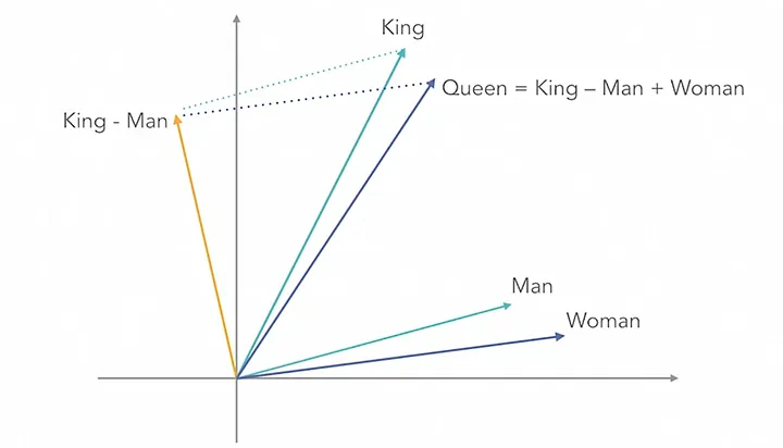
The idea is simple:

• Every word becomes a point in a high-dimensional space.

• Similar words appear close together.

• Relationships become directions in that space.

Why One-Hot Encoding Is Not Enough

Consider:

cat, dog, horse, computer

Using one-hot encoding:

cat      = [1,0,0,0]
dog      = [0,1,0,0]
horse    = [0,0,1,0]
computer = [0,0,0,1]

Problems:

• High-dimensional

• Sparse

• No semantic information

• Every pair of words is equally distant

import numpy as np

vocab = ["cat", "dog", "horse", "computer"]

for i, word in enumerate(vocab):
    vec = np.zeros(len(vocab))
    vec[i] = 1
    print(word, vec)

cat [1. 0. 0. 0.]
dog [0. 1. 0. 0.]
horse [0. 0. 1. 0.]
computer [0. 0. 0. 1.]

Problems with One-Hot Encoding:

1. High Dimensionality: For a vocabulary of 100,000 words, each vector has 100,000 dimensions

2. No Semantic Information: The angle between “cat” and “dog” is the same as “cat” and “refrigerator”

3. Sparse Vectors: Almost all values are zero, leading to inefficient computation

The Solution: Dense Word Embeddings

Word embeddings solve these problems by representing each word as a dense vector (typically 100-300 dimensions) where semantically similar words have similar vectors.

cat    → [0.23, -0.45, 0.67, ..., 0.12]  (300 dimensions)
dog    → [0.25, -0.42, 0.65, ..., 0.15]  (300 dimensions)
refrigerator → [-0.89, 0.34, -0.12, ..., -0.56]

Now, the vectors for “cat” and “dog” are close together, while “refrigerator” is far away!

The Distributional Hypothesis

The foundation of Word2Vec is:

You shall know a word by the company it keeps.

— J. R. Firth

Example:

The cat chased the mouse.
The dog chased the ball.

Because cat and dog occur in similar contexts, Word2Vec tends to learn similar representations for them.

Intuitive Example: Animal Space

Let’s build an intuitive understanding by creating a simple 2D “animal space” based on two characteristics: cuteness and size (both on a scale of 0-100).

import matplotlib.pyplot as plt

animals = {
    'kitten': [95, 10],
    'hamster': [90, 8],
    'puppy': [92, 15],
    'cat': [75, 25],
    'dog': [60, 40],
    'chicken': [30, 20],
    'horse': [40, 70],
    'elephant': [50, 95],
    'tarantula': [5, 10]
}

# Plot animals
fig, ax = plt.subplots(figsize=(10, 7))
for animal, (cute, size) in animals.items():
    ax.scatter(size, cute, s=200)
    ax.annotate(animal, (size, cute), xytext=(5, 5), textcoords='offset points')

ax.set_xlabel('Size →', fontsize=12)
ax.set_ylabel('Cuteness →', fontsize=12)
ax.set_title('Animal Space (2D Word Embeddings)', fontsize=14)
ax.set_xlim(-5, 105)
ax.set_ylim(-5, 105)
ax.grid(True, alpha=0.3)
plt.show()

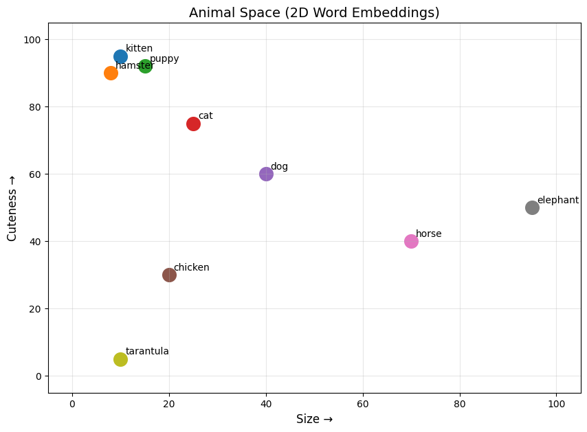
In this 2D space:

• Kitten and hamster are close (both small and cute)

• Elephant is isolated (very large, moderately cute)

• Horse is between small and large animals

Vector Operations Reveal Semantic Relationships

The power of word embeddings comes from vector arithmetic. Remember the king-man example.

Word2Vec and Encoder–Decoder Models

In Lecture 8 we studied encoder–decoder architectures.

Word2Vec can be viewed as a very simple encoder–decoder model.

Word
 ↓
Encoder
 ↓
Latent Representation
 ↓
Decoder
 ↓
Context Prediction

Autoencoder vs Word2Vec

Autoencoder	Word2Vec
Reconstructs input	Predicts context
Learns latent code	Learns word embedding
Input = target	Input ≠ target
Compression	Semantic representation

The embedding vector plays a role similar to the latent representation in an autoencoder.

---

Practical Examples with Pre-trained Models

Loading Pre-trained Word Vectors

We’ll use Gensim to load pre-trained word vectors. First, install the required package:

# Install gensim 
# !pip install gensim

import numpy as np
import gensim.downloader as api

c:\Users\m.amintoosi\.conda\envs\pth-gpu\lib\site-packages\google\api_core\_python_version_support.py:263: FutureWarning: You are using a Python version (3.10.16) which Google will stop supporting in new releases of google.api_core once it reaches its end of life (2026-10-04). Please upgrade to the latest Python version, or at least Python 3.11, to continue receiving updates for google.api_core past that date.
  warnings.warn(message, FutureWarning)

# Load pre-trained GloVe vectors (100-dimensional, trained on Wikipedia)
# This will download the model on first run (~128 MB)
print("Loading pre-trained word vectors...")
model = api.load("glove-wiki-gigaword-100")
print(f"Loaded {len(model.key_to_index):,} word vectors")

Loading pre-trained word vectors...
Loaded 400,000 word vectors

# Examine a word vector
print(f"Vector for 'king' (first 10 dimensions): {model['king'][:10]}")
print(f"Vector shape: {model['king'].shape}")

Vector for 'king' (first 10 dimensions): [-0.32307 -0.87616  0.21977  0.25268  0.22976  0.7388  -0.37954 -0.35307
 -0.84369 -1.1113 ]
Vector shape: (100,)

Finding Similar Words

# Find the 10 most similar words to "king"
similar_to_king = model.most_similar("king", topn=5)

print("Words most similar to 'king':")
for word, similarity in similar_to_king:
    print(f"  {word:15} → {similarity:.4f}")

Words most similar to 'king':
  prince          → 0.7682
  queen           → 0.7508
  son             → 0.7021
  brother         → 0.6986
  monarch         → 0.6978

# Try with other words
for query_word in ["computer", "beautiful", "iran", "tehran"]:
    if query_word in model.key_to_index:
        print(f"\nWords similar to '{query_word}':")
        for word, sim in model.most_similar(query_word, topn=5):
            print(f"  {word:15} {sim:.4f}")
    else:
        print(f"'{query_word}' not in vocabulary")

Words similar to 'computer':
  computers       0.8752
  software        0.8373
  technology      0.7642
  pc              0.7366
  hardware        0.7290

Words similar to 'beautiful':
  lovely          0.8909
  gorgeous        0.8722
  wonderful       0.8081
  charming        0.7719
  magnificent     0.7332

Words similar to 'iran':
  tehran          0.8503
  iranian         0.7911
  syria           0.7800
  iraq            0.7679
  nuclear         0.7258

Words similar to 'tehran':
  iran            0.8503
  iranian         0.7557
  pyongyang       0.7014
  ahmadinejad     0.6929
  moscow          0.6898

The Famous Analogy: King - Man + Woman = Queen

This is the most famous example of word vector arithmetic. The idea is:

If we take the concept of “king,” remove the “maleness,” and add “femaleness,” we should get “queen.”

# The classic analogy: king - man + woman = ?
result = model.most_similar(positive=['king', 'woman'], negative=['man'], topn=5)

print("king - man + woman = ?")
print("-" * 40)
for word, similarity in result:
    print(f"  {word:15} → {similarity:.4f}")

king - man + woman = ?
----------------------------------------
  queen           → 0.7699
  monarch         → 0.6843
  throne          → 0.6756
  daughter        → 0.6595
  princess        → 0.6521

Queen is the top result! The vector arithmetic successfully captures the gender relationship.

Understanding the Math Behind Analogies

def explain_analogy(word_a, word_b, word_c, model):
    """
    Analogy: word_a is to word_b as word_c is to ?
    
    Mathematically: ? ≈ word_b - word_a + word_c
    """
    # Get vectors
    vec_a = model[word_a]
    vec_b = model[word_b]
    vec_c = model[word_c]
    
    # Compute the target vector
    target_vec = vec_b - vec_a + vec_c
    
    # Find closest words
    results = model.most_similar(positive=[word_b, word_c], negative=[word_a], topn=5)
    
    print(f"Analogy: {word_a} is to {word_b} as {word_c} is to ?")
    print(f"\nMathematical operation:")
    print(f"  target = {word_b} - {word_a} + {word_c}")
    print(f"  target = {vec_b[:3]}... - {vec_a[:3]}... + {vec_c[:3]}...")
    print(f"  target = {target_vec[:3]}...")
    print(f"\nTop predictions:")
    for word, sim in results:
        print(f"  {word}: {sim:.4f}")
    
    return results

# Run the explanation
explain_analogy("man", "king", "woman", model)

Analogy: man is to king as woman is to ?

Mathematical operation:
  target = king - man + woman
  target = [-0.32307 -0.87616  0.21977]... - [0.37293 0.38503 0.71086]... + [0.59368 0.44825 0.5932 ]...
  target = [-0.10231996 -0.81294006  0.10211003]...

Top predictions:
  queen: 0.7699
  monarch: 0.6843
  throne: 0.6756
  daughter: 0.6595
  princess: 0.6521

[('queen', 0.7698540687561035),
 ('monarch', 0.6843381524085999),
 ('throne', 0.6755736470222473),
 ('daughter', 0.6594556570053101),
 ('princess', 0.6520534157752991)]

More Analogy Examples

def run_analogy(positive, negative, topn=5):
    """Helper function to run analogies."""
    results = model.most_similar(positive=positive, negative=negative, topn=topn)
    formula = " + ".join(positive)
    if negative:
        formula += " - " + " - ".join(negative)
    print(f"{formula} = ?")
    for word, sim in results:
        print(f"  {word}: {sim:.4f}")
    print()

# Geographic analogies
print("=" * 50)
print("GEOGRAPHIC ANALOGIES")
print("=" * 50)
run_analogy(['paris', 'japan'], ['france'])
run_analogy(['tehran', 'germany'], ['iran'])

# Grammatical analogies
print("=" * 50)
print("GRAMMATICAL ANALOGIES")
print("=" * 50)
run_analogy(['walking', 'swim'], ['walk'])
run_analogy(['mice', 'dog'], ['mouse'])

# Semantic analogies
print("=" * 50)
print("SEMANTIC ANALOGIES")
print("=" * 50)
run_analogy(['summer', 'cold'], ['winter'])
run_analogy(['doctor', 'law'], ['hospital'])

==================================================
GEOGRAPHIC ANALOGIES
==================================================
paris + japan - france = ?
  tokyo: 0.8994
  osaka: 0.7421
  japanese: 0.7059
  seoul: 0.6949
  shanghai: 0.6679

tehran + germany - iran = ?
  berlin: 0.8361
  munich: 0.7773
  frankfurt: 0.7377
  cologne: 0.7185
  hamburg: 0.7169

==================================================
GRAMMATICAL ANALOGIES
==================================================

walking + swim - walk = ?
  swimming: 0.8009
  surfing: 0.6603
  swam: 0.6448
  rowing: 0.6413
  jogging: 0.6376

mice + dog - mouse = ?
  dogs: 0.8048
  rats: 0.7038
  cats: 0.6896
  animals: 0.6468
  horses: 0.6444

==================================================
SEMANTIC ANALOGIES
==================================================
summer + cold - winter = ?
  hot: 0.7388
  cool: 0.6947
  warm: 0.6855
  days: 0.6771
  turned: 0.6674

doctor + law - hospital = ?
  laws: 0.7347
  subject: 0.6480
  statute: 0.6445
  rules: 0.6442
  legal: 0.6344

Finding the Odd One Out

# Find the word that doesn't belong
words_list1 = ["breakfast", "cereal", "dinner", "lunch"]
words_list2 = ["dog", "cat", "car", "fish"]
words_list3 = ["apple", "orange", "banana", "car"]

print("Which word doesn't belong?")
print(f"  {words_list1} → {model.doesnt_match(words_list1)}")
print(f"  {words_list2} → {model.doesnt_match(words_list2)}")
print(f"  {words_list3} → {model.doesnt_match(words_list3)}")

Which word doesn't belong?
  ['breakfast', 'cereal', 'dinner', 'lunch'] → cereal
  ['dog', 'cat', 'car', 'fish'] → car
  ['apple', 'orange', 'banana', 'car'] → car

Computing Similarity Scores

# Compute similarity between word pairs
word_pairs = [
    ("king", "queen"),
    ("king", "man"),
    ("king", "apple"),
    ("dog", "puppy"),
    ("dog", "cat"),
    ("happy", "sad"),
    ("fast", "quick"),
    ("big", "small"),
]

print("Word Pair Similarities:")
print("-" * 45)
for w1, w2 in word_pairs:
    sim = model.similarity(w1, w2)
    print(f"  {w1:10} ↔ {w2:10} : {sim:.4f}")

Word Pair Similarities:
---------------------------------------------
  king       ↔ queen      : 0.7508
  king       ↔ man        : 0.5119
  king       ↔ apple      : 0.2668
  dog        ↔ puppy      : 0.7236
  dog        ↔ cat        : 0.8798
  happy      ↔ sad        : 0.6801
  fast       ↔ quick      : 0.7107
  big        ↔ small      : 0.7180

Interesting observation: Antonyms like “big” and “small” often have high similarity because they appear in similar contexts (e.g., “How big/small is it?”). This shows that word embeddings capture distributional similarity, not necessarily semantic similarity in the traditional sense.

Simple Query: “Capital of Iran”

# Find the capital of Iran
# Logic: If paris is to france as X is to iran
# X = paris - france + iran

result = model.most_similar(positive=['paris', 'iran'], negative=['france'], topn=5)

print("Query: What is the capital of Iran?")
print("  paris - france + iran = ?")
print("-" * 40)
for word, sim in result:
    print(f"  {word}: {sim:.4f}")

Query: What is the capital of Iran?
  paris - france + iran = ?
----------------------------------------
  tehran: 0.8785
  iranian: 0.7055
  moscow: 0.6929
  seoul: 0.6468
  cairo: 0.6466

Visualizing Word Relationships (t-SNE)

from sklearn.manifold import TSNE
import matplotlib.pyplot as plt

# Select interesting words
words_of_interest = [
    'king', 'queen', 'prince', 'princess', 'man', 'woman',
    'paris', 'france', 'berlin', 'germany', 'rome', 'italy',
    'cat', 'dog', 'fish', 'bird', 'horse', 'elephant',
    'good', 'bad', 'happy', 'sad', 'big', 'small',
    'doctor', 'nurse', 'hospital', 'medicine'
]

# Filter to words that exist in the model
words_of_interest = [w for w in words_of_interest if w in model.key_to_index]

# Get vectors for these words
word_vectors = np.array([model[w] for w in words_of_interest])

# Reduce to 2D using t-SNE
tsne = TSNE(n_components=2, random_state=42, perplexity=min(15, len(words_of_interest)-1))
word_vectors_2d = tsne.fit_transform(word_vectors)

# Plot
plt.figure(figsize=(14, 10))
plt.scatter(word_vectors_2d[:, 0], word_vectors_2d[:, 1], c='blue', alpha=0.5)

for i, word in enumerate(words_of_interest):
    plt.annotate(word, (word_vectors_2d[i, 0], word_vectors_2d[i, 1]), 
                 fontsize=10, ha='center', va='bottom')

plt.title("Word Embeddings Visualized with t-SNE", fontsize=14)
plt.xlabel("t-SNE Dimension 1")
plt.ylabel("t-SNE Dimension 2")
plt.grid(True, alpha=0.3)
plt.tight_layout()
plt.show()

c:\Users\m.amintoosi\.conda\envs\pth-gpu\lib\site-packages\joblib\externals\loky\backend\context.py:136: UserWarning: Could not find the number of physical cores for the following reason:
[WinError 2] The system cannot find the file specified
Returning the number of logical cores instead. You can silence this warning by setting LOKY_MAX_CPU_COUNT to the number of cores you want to use.
  warnings.warn(
  File "c:\Users\m.amintoosi\.conda\envs\pth-gpu\lib\site-packages\joblib\externals\loky\backend\context.py", line 257, in _count_physical_cores
    cpu_info = subprocess.run(
  File "c:\Users\m.amintoosi\.conda\envs\pth-gpu\lib\subprocess.py", line 503, in run
    with Popen(*popenargs, **kwargs) as process:
  File "c:\Users\m.amintoosi\.conda\envs\pth-gpu\lib\subprocess.py", line 971, in __init__
    self._execute_child(args, executable, preexec_fn, close_fds,
  File "c:\Users\m.amintoosi\.conda\envs\pth-gpu\lib\subprocess.py", line 1456, in _execute_child
    hp, ht, pid, tid = _winapi.CreateProcess(executable, args,

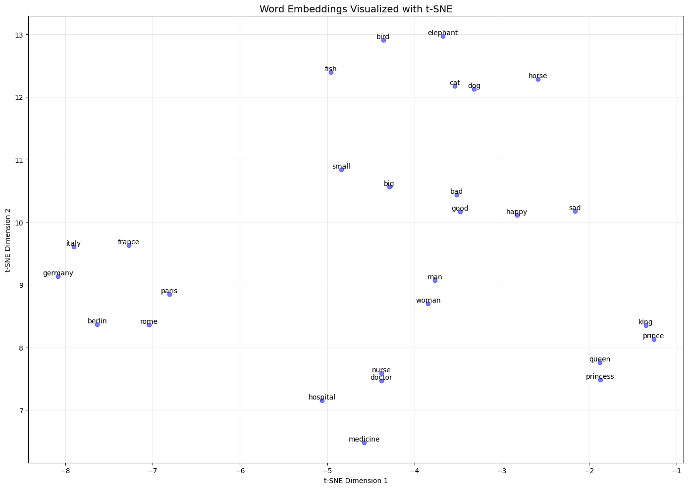
Observations from the visualization:

• Royalty words (king, queen, prince, princess) cluster together

• Country-capital pairs (paris-france, berlin-germany) are near each other

• Animals form their own cluster

• Antonyms (good-bad, happy-sad, big-small) are relatively close but in opposite directions

Predicting Context

Consider:

the cat sat on the mat

Window size = 2

Center word:

sat

Context words:

cat
on
the
mat

Source

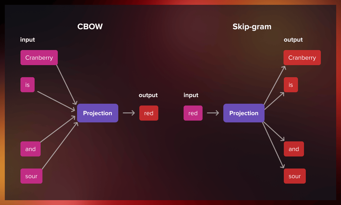
Skip-Gram Training Examples

(sat → cat)
(sat → on)
(sat → the)
(sat → mat)

Skip-Gram Architecture

Source

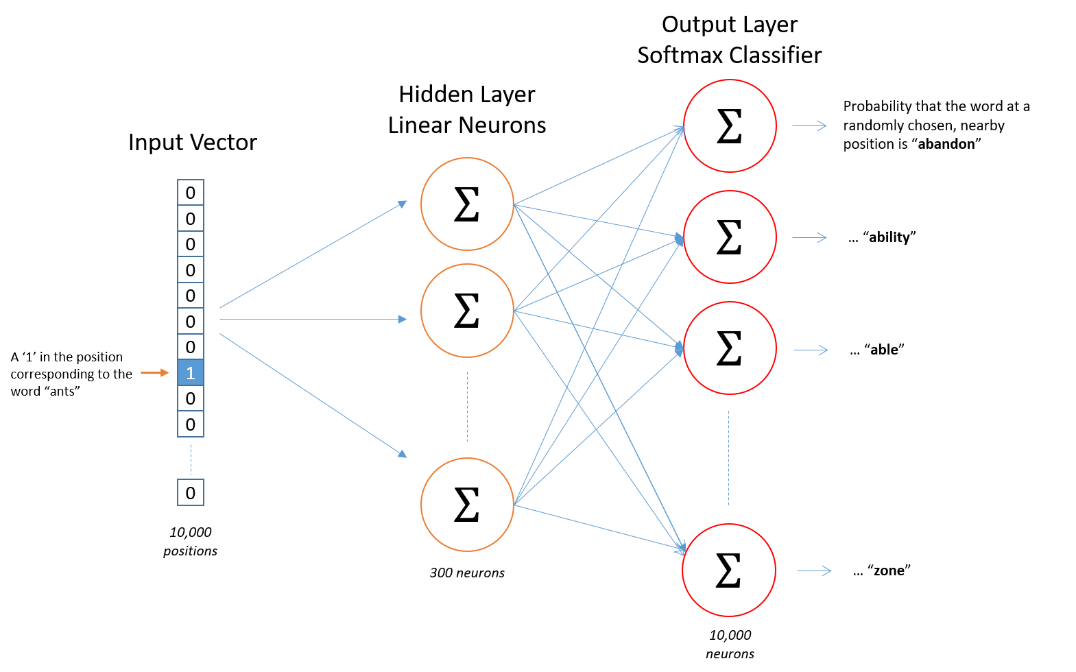
Generating Training Examples

sentence = "Anne was beginning to get very tired".split()

window_size = 2

for i, center_word in enumerate(sentence):

    start = max(0, i-window_size)
    end = min(len(sentence), i+window_size+1)

    context = [
        sentence[j]
        for j in range(start, end)
        if j != i
    ]

    print(center_word, "->", context)

Anne -> ['was', 'beginning']
was -> ['Anne', 'beginning', 'to']
beginning -> ['Anne', 'was', 'to', 'get']
to -> ['was', 'beginning', 'get', 'very']
get -> ['beginning', 'to', 'very', 'tired']
very -> ['to', 'get', 'tired']
tired -> ['get', 'very']

For the center word beginning, the generated training pairs are:

(beginning → Anne)
(beginning → was)
(beginning → to)
(beginning → get)

Loading Anne of Green Gables

We now move from toy examples to a real corpus.

data/Anne_of_Green_Gables.txt

from pathlib import Path
import re

corpus_path = Path("data/Anne_of_Green_Gables.txt")

text = corpus_path.read_text(
    encoding="utf-8"
)

text = text.lower()
text = re.sub(r"[^a-z\s]", " ", text)

tokens = text.split()

print("Number of tokens:", len(tokens))

Number of tokens: 107178

from collections import Counter

Counter(tokens).most_common(20)

[('the', 3926),
 ('and', 3398),
 ('i', 3265),
 ('to', 3046),
 ('a', 2229),
 ('it', 2099),
 ('of', 1923),
 ('you', 1702),
 ('she', 1519),
 ('in', 1479),
 ('that', 1371),
 ('was', 1364),
 ('her', 1315),
 ('anne', 1214),
 ('t', 1189),
 ('s', 1153),
 ('marilla', 851),
 ('but', 849),
 ('be', 822),
 ('as', 791)]

Training Word2Vec with Gensim

Instead of implementing Word2Vec from scratch, we use a well-tested implementation.

from gensim.models import Word2Vec

sentences = [tokens]

model = Word2Vec(
    sentences=sentences,
    vector_size=100,
    window=5,
    min_count=5,
    sg=1,
    epochs=10
)

Important Hyperparameters

• vector_size : embedding dimension

• window : context window size

• min_count : minimum frequency

• sg=1 : Skip-Gram

• sg=0 : CBOW

Exploring the Learned Embeddings

model.wv.most_similar("anne", topn=5)

[('surprised', 0.9965387582778931),
 ('concert', 0.9963647127151489),
 ('confession', 0.9953275322914124),
 ('invited', 0.9946743249893188),
 ('school', 0.9944130778312683)]

model.wv.most_similar("marilla", topn=5)

[('herself', 0.993959903717041),
 ('head', 0.9935182332992554),
 ('door', 0.993461549282074),
 ('sorrel', 0.9931078553199768),
 ('came', 0.9930408000946045)]

model.wv.similarity("anne", "matthew")

0.9744315

Analogy Tasks

The famous analogy examples can be tested using vector arithmetic.

# model.wv.most_similar(
#     positive=["king", "woman"],
#     negative=["man"],
#     topn=5
# )

Because Anne of Green Gables is relatively small, these analogies may not work. This is an important lesson:

Better embeddings usually require larger corpora.

Character Visualization

A particularly interesting activity is to visualize embeddings for:

• Anne

• Marilla

• Matthew

• Diana

• Gilbert

• Miss Stacy (Stacey)

and investigate whether characters with similar narrative roles cluster together.

Source

Figure Source

Pretrained Embeddings with spaCy

Our corpus is relatively small.

Modern NLP systems often use embeddings trained on billions of words.

# !pip install spacy
# !python -m spacy download en_core_web_md

import spacy

nlp = spacy.load("en_core_web_md")

Now let’s revisit the examples from the beginning of the lecture.

nlp("king").similarity(nlp("queen"))

0.3825309165573663

nlp("man").similarity(nlp("woman"))

0.15610169391657686

nlp("paris").similarity(nlp("tehran"))

0.5575575739852713

nlp("cat").similarity(nlp("dog"))

1.0000000568192473

import spacy
import numpy as np

# Test if vectors are working
nlp = spacy.load("en_core_web_md")  # Must be md or lg!

# Quick sanity check
king_vec = nlp("king").vector
queen_vec = nlp("queen").vector

similarity = np.dot(king_vec, queen_vec) / (np.linalg.norm(king_vec) * np.linalg.norm(queen_vec))
print(f"King-Queen similarity: {similarity:.4f}")
print(f"Vector shape: {king_vec.shape}")

# This should output something like:
# King-Queen similarity: 0.6512
# Vector shape: (100,) or (300,)

King-Queen similarity: 0.3825
Vector shape: (300,)

import spacy
import numpy as np

# Load the model with vectors (must be md or lg)
try:
    nlp = spacy.load("en_core_web_md")
    print("Loaded en_core_web_md successfully!")
except OSError:
    print("Model not found. Download with: python -m spacy download en_core_web_md")
    exit()

def cosine_similarity(vec1, vec2):
    """Calculate cosine similarity between two vectors"""
    if np.linalg.norm(vec1) == 0 or np.linalg.norm(vec2) == 0:
        return 0
    return np.dot(vec1, vec2) / (np.linalg.norm(vec1) * np.linalg.norm(vec2))

def analogy(a, b, c, topn=5):
    """
    Solve analogy: a : b :: c : ?
    Example: man : king :: woman : queen
    """
    # Get word vectors
    vec_a = nlp(a).vector
    vec_b = nlp(b).vector
    vec_c = nlp(c).vector
    
    # Target vector: b - a + c
    target = vec_b - vec_a + vec_c
    
    # Find closest words
    results = []
    for token in nlp.vocab:
        # Filter: only real words with vectors
        if (token.has_vector and token.is_alpha and token.is_lower and 
            len(token.text) > 1 and token.text not in [a, b, c]):
            sim = cosine_similarity(target, token.vector)
            results.append((token.text, sim))
    
    results.sort(key=lambda x: x[1], reverse=True)
    return results[:topn]

def check_vector_quality():
    """Check if vectors are meaningful"""
    test_words = ["king", "queen", "man", "woman"]
    print("\nChecking vector quality:")
    print("-" * 40)
    
    for word in test_words:
        if nlp(word).has_vector:
            print(f"✓ '{word}' has vector (norm: {np.linalg.norm(nlp(word).vector):.2f})")
        else:
            print(f"✗ '{word}' has NO vector - using wrong model!")
    
    # Test basic similarity
    king_vec = nlp("king").vector
    queen_vec = nlp("queen").vector
    sim = cosine_similarity(king_vec, queen_vec)
    print(f"\nSimilarity between 'king' and 'queen': {sim:.4f}")
    print("(Should be ~0.6-0.7 for a good model)")

# First, check if vectors are working
check_vector_quality()

print("\n" + "="*60)
print("FAMOUS WORD ANALOGIES")
print("="*60)

# Test 1: King - Man + Woman
print("\n1. King : Man :: Queen : Woman")
print("-" * 40)
results = analogy("man", "king", "woman")
print(f"   Top result: {results[0][0]} (score: {results[0][1]:.4f})")
print(f"   Top 5 results: {[w for w, _ in results[:5]]}")

# Test 2: Paris - France + Germany
print("\n2. Paris : France :: Berlin : Germany")
print("-" * 40)
results = analogy("france", "paris", "germany")
print(f"   Top result: {results[0][0]} (score: {results[0][1]:.4f})")
print(f"   Top 5 results: {[w for w, _ in results[:5]]}")

# Test 3: Walking - Walk + Sleep
print("\n3. Walking : Walk :: Sleeping : Sleep")
print("-" * 40)
results = analogy("walk", "walking", "sleep")
print(f"   Top result: {results[0][0]} (score: {results[0][1]:.4f})")

# Test 4: Better - Good + Bad
print("\n4. Better : Good :: Worse : Bad")
print("-" * 40)
results = analogy("good", "better", "bad")
print(f"   Top result: {results[0][0]} (score: {results[0][1]:.4f})")

# Verification
print("\n" + "="*60)
print("VERIFYING THE RELATIONSHIP")
print("="*60)

vec_king = nlp("king").vector
vec_man = nlp("man").vector
vec_queen = nlp("queen").vector
vec_woman = nlp("woman").vector

vec1 = vec_king - vec_man
vec2 = vec_queen - vec_woman
similarity = cosine_similarity(vec1, vec2)
print(f"Similarity between (king - man) and (queen - woman): {similarity:.4f}")
print(f"Perfect analogy would be near 1.0, actual: {similarity:.4f}")

Loaded en_core_web_md successfully!

Checking vector quality:
----------------------------------------
✓ 'king' has vector (norm: 6.87)
✓ 'queen' has vector (norm: 7.02)
✓ 'man' has vector (norm: 7.14)
✓ 'woman' has vector (norm: 8.12)

Similarity between 'king' and 'queen': 0.3825
(Should be ~0.6-0.7 for a good model)

============================================================
FAMOUS WORD ANALOGIES
============================================================

1. King : Man :: Queen : Woman
----------------------------------------
   Top result: queen (score: 0.4812)
   Top 5 results: ['queen', 'll', 'got', 'has', 'lovin']

2. Paris : France :: Berlin : Germany
----------------------------------------
   Top result: co (score: 0.2790)
   Top 5 results: ['co', 've', 'woman', 'lovin', 'ol']

3. Walking : Walk :: Sleeping : Sleep
----------------------------------------
   Top result: had (score: 0.4569)

4. Better : Good :: Worse : Bad
----------------------------------------
   Top result: would (score: 1.0000)

============================================================
VERIFYING THE RELATIONSHIP
============================================================
Similarity between (king - man) and (queen - woman): 0.0146
Perfect analogy would be near 1.0, actual: 0.0146

The pretrained spaCy vectors usually capture semantic relationships much better than embeddings trained on a single novel.

Gensim vs spaCy

Gensim	spaCy
Train embeddings	Usually uses pretrained embeddings
Educational & Research	Production NLP
Corpus-specific models	General-purpose models
Full control over training	Convenient & ready-to-use
Word2Vec, Doc2Vec, FastText	Word vectors, Contextual vectors
Excellent for word analogies	Not suitable for analogies
Requires large text corpus for training	Works out-of-box with small models
Lower-level access to vectors	Higher-level NLP pipeline
Best for topic modeling (LDA)	Best for NER, POS tagging, Dependency parsing
Slower inference	Optimized for speed
No built-in tokenization	Advanced tokenization & lemmatization
Manual preprocessing needed	Built-in preprocessing pipeline
Ideal for semantic similarity tasks	Ideal for syntactic & structural analysis
Models can be 1-3GB+	Small models as low as 11MB
Community-driven	Industry-driven (Explosion AI)
Python + NumPy backend	Python + Cython backend (fast)
Great for custom embeddings	Great for transfer learning (spaCy transformers)

Additional Comparison Points

Feature	Gensim	spaCy
Primary Use Case	Unsupervised semantic modeling	Production-ready NLP pipeline
Learning Curve	Steeper (requires ML knowledge)	Gentle (API-focused)
Documentation	Academic-style	Industry/developer-friendly
Pre-trained Models	Many (GloVe, Word2Vec, FastText)	Fewer but high quality
Multilingual Support	Limited	Excellent (70+ languages)
Training Speed	Fast (optimized C routines)	Moderate
Memory Usage	High (full vectors in memory)	Low to moderate
Batch Processing	Excellent (streaming)	Good
Integration	Standalone	Integrates with DL frameworks

When to Use Which

Scenario	Best Choice	Reason
Word analogies (king - man + woman)	Gensim	Built-in most_similar() with positive/negative
Named Entity Recognition	spaCy	State-of-the-art pre-trained NER
Training custom word vectors	Gensim	Full control over Word2Vec parameters
Part-of-Speech tagging	spaCy	Accurate out-of-box POS tagging
Topic modeling	Gensim	Native LDA, HDP, etc.
Dependency parsing	spaCy	Excellent syntactic parsing
Large-scale document similarity	Gensim	Memory-efficient similarity queries
Quick NLP prototype	spaCy	One-liner for common tasks
Academic research on embeddings	Gensim	Reproducible, parameter transparency
Production API service	spaCy	Fast, reliable, low latency

Code Example Comparison

# GENSIM - Word embeddings & analogies
import gensim.downloader as api
model = api.load("glove-wiki-gigaword-300")
similarity = model.similarity("king", "queen")  # 0.65
result = model.most_similar(positive=["king", "woman"], negative=["man"])

# SPACY - NLP pipeline
import spacy
nlp = spacy.load("en_core_web_sm")
doc = nlp("Apple is looking to buy U.K. startup for $1 billion")
for ent in doc.ents:
    print(ent.label_, ent.text)  # ORG Apple, GPE U.K., MONEY $1 billion

Performance Comparison

Metric	Gensim	spaCy
Load time (medium model)	5-10 seconds	2-3 seconds
Inference speed	Moderate	Fast
Memory footprint	1-3 GB	100 MB - 1 GB
Training time (1M sentences)	10-30 minutes	N/A (uses pretrained)

Summary Recommendation

• Use Gensim when: You need word analogies, topic modeling, or training custom embeddings on your own corpus

• Use spaCy when: You need a complete NLP pipeline (NER, POS, parsing) for production applications

• Use both when: You want to extract features with spaCy and then train embeddings with Gensim

From Word2Vec to Transformers

Word2Vec produces static embeddings.

bank → one vector

regardless of context.

Place a figure in:

Figure Source

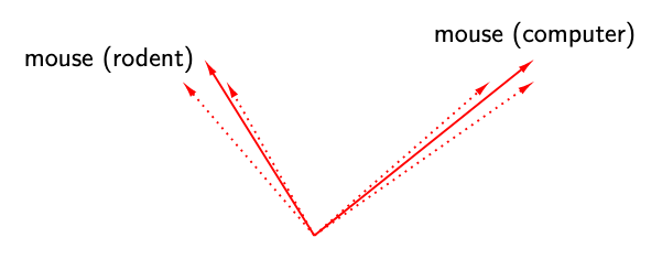
Consider:

I deposited money in the bank.

The fisherman sat by the bank.

Word2Vec:

same vector

Transformer models (BERT, GPT, RoBERTa):

different vectors

because the representation depends on context.

Historical Perspective

One-Hot Encoding
        ↓
Word2Vec
        ↓
GloVe
        ↓
FastText
        ↓
BERT
        ↓
GPT Embeddings

Summary

In this notebook we:

• Motivated word embeddings using famous analogy examples.

• Studied the distributional hypothesis.

• Connected Word2Vec to encoder–decoder architectures.

• Learned Skip-Gram and CBOW.

• Generated training examples.

• Trained Word2Vec on Anne of Green Gables.

• Explored similarity and analogy queries.

• Visualized embeddings using t-SNE.

• Used pretrained embeddings with spaCy.

• Connected Word2Vec to modern transformer embeddings.

Word2Vec remains one of the most influential ideas in deep learning because it demonstrated that meaningful semantic representations can emerge from self-supervised prediction tasks.