


Appendix H: Transposed Convolution#
The CNN layers we have seen so far, such as convolutional layers and pooling layers, typically reduce (downsample) the spatial dimensions (height and width) of the input, or keep them unchanged. In semantic segmentation that classifies at pixel-level, it will be convenient if the spatial dimensions of the input and output are the same. For example, the channel dimension at one output pixel can hold the classification results for the input pixel at the same spatial position.
To achieve this, especially after the spatial dimensions are reduced by CNN layers, we can use another type of CNN layers that can increase (upsample) the spatial dimensions of intermediate feature maps. In this section, we will introduce transposed convolution, which is also called fractionally-strided convolution, for reversing downsampling operations by the convolution.
import torch
from torch import nn
# from d2l import torch as d2l
Basic Operation#
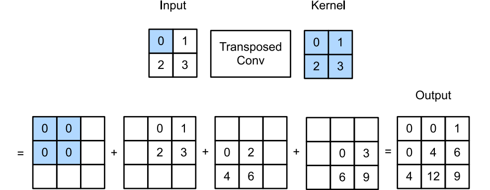
Ignoring channels for now, let’s begin with the basic transposed convolution operation with stride of 1 and no padding. Suppose that we are given a \(n_h \times n_w\) input tensor and a \(k_h \times k_w\) kernel. Sliding the kernel window with stride of 1 for \(n_w\) times in each row and \(n_h\) times in each column yields a total of \(n_h n_w\) intermediate results. Each intermediate result is a \((n_h + k_h - 1) \times (n_w + k_w - 1)\) tensor that are initialized as zeros. To compute each intermediate tensor, each element in the input tensor is multiplied by the kernel so that the resulting \(k_h \times k_w\) tensor replaces a portion in each intermediate tensor. Note that the position of the replaced portion in each intermediate tensor corresponds to the position of the element in the input tensor used for the computation. In the end, all the intermediate results are summed over to produce the output.
As an example, the following figure illustrates how transposed convolution with a \(2\times 2\) kernel is computed for a \(2\times 2\) input tensor.
We can (implement this basic transposed convolution operation) trans_conv for a input matrix X and a kernel matrix K.
def trans_conv(X, K):
    h, w = K.shape
    Y = torch.zeros((X.shape[0] + h - 1, X.shape[1] + w - 1))
    for i in range(X.shape[0]):
        for j in range(X.shape[1]):
            Y[i: i + h, j: j + w] += X[i, j] * K
    return Y
In contrast to the regular convolution (in :numref:sec_conv_layer) that reduces input elements
via the kernel,
the transposed convolution
broadcasts input elements
via the kernel, thereby
producing an output
that is larger than the input.
We can construct the input tensor X and the kernel tensor K from :numref:fig_trans_conv to validate the output of the above implementation of the basic two-dimensional transposed convolution operation.
X = torch.tensor([[0.0, 1.0], [2.0, 3.0]])
K = torch.tensor([[0.0, 1.0], [2.0, 3.0]])
trans_conv(X, K)
tensor([[ 0.,  0.,  1.],
        [ 0.,  4.,  6.],
        [ 4., 12.,  9.]])
Alternatively,
when the input X and kernel K are both
four-dimensional tensors,
we can use high-level APIs to obtain the same results.
X, K = X.reshape(1, 1, 2, 2), K.reshape(1, 1, 2, 2)
tconv = nn.ConvTranspose2d(1, 1, kernel_size=2, bias=False)
tconv.weight.data = K
tconv(X)
tensor([[[[ 0.,  0.,  1.],
          [ 0.,  4.,  6.],
          [ 4., 12.,  9.]]]], grad_fn=<ConvolutionBackward0>)
Padding, Strides, and Multiple Channels#
Different from in the regular convolution where padding is applied to input, it is applied to output in the transposed convolution. For example, when specifying the padding number on either side of the height and width as 1, the first and last rows and columns will be removed from the transposed convolution output.
tconv = nn.ConvTranspose2d(1, 1, kernel_size=2, padding=1, bias=False)
tconv.weight.data = K
tconv(X)
tensor([[[[4.]]]], grad_fn=<ConvolutionBackward0>)
In the transposed convolution, strides are specified for intermediate results (thus output), not for input. Using the same input and kernel tensors as before, changing the stride from 1 to 2 increases both the height and weight of intermediate tensors, hence the output tensor in the following figure.
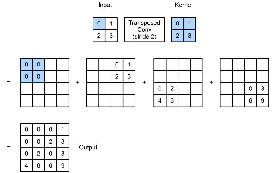
The following code snippet can validate the transposed convolution output for stride of 2.
tconv = nn.ConvTranspose2d(1, 1, kernel_size=2, stride=2, bias=False)
tconv.weight.data = K
tconv(X)
tensor([[[[0., 0., 0., 1.],
          [0., 0., 2., 3.],
          [0., 2., 0., 3.],
          [4., 6., 6., 9.]]]], grad_fn=<ConvolutionBackward0>)
For multiple input and output channels, the transposed convolution works in the same way as the regular convolution. Suppose that the input has \(c_i\) channels, and that the transposed convolution assigns a \(k_h\times k_w\) kernel tensor to each input channel. When multiple output channels are specified, we will have a \(c_i\times k_h\times k_w\) kernel for each output channel.
As in all, if we feed \(\mathsf{X}\) into a convolutional layer \(f\) to output \(\mathsf{Y}=f(\mathsf{X})\) and create a transposed convolutional layer \(g\) with the same hyperparameters as \(f\) except for the number of output channels being the number of channels in \(\mathsf{X}\), then \(g(Y)\) will have the same shape as \(\mathsf{X}\). This can be illustrated in the following example.
X = torch.rand(size=(1, 10, 16, 16))
conv = nn.Conv2d(10, 20, kernel_size=5, padding=2, stride=3)
tconv = nn.ConvTranspose2d(20, 10, kernel_size=5, padding=2, stride=3)
tconv(conv(X)).shape == X.shape
True
Connection to Matrix Transposition#
The transposed convolution is named after
the matrix transposition.
To explain,
let’s first
see how to implement convolutions
using matrix multiplications.
In the example below, we define a \(3\times 3\) input X and a \(2\times 2\) convolution kernel K, and then use the corr2d function to compute the convolution output Y.
from scipy import signal

X = torch.arange(9.0).reshape(3, 3)
K = torch.tensor([[1.0, 2.0], [3.0, 4.0]])
# Y = d2l.corr2d(X, K)
Y = signal.correlate2d(X, K, mode="valid")
print(X)
print(K)
print(Y)
tensor([[0., 1., 2.],
        [3., 4., 5.],
        [6., 7., 8.]])
tensor([[1., 2.],
        [3., 4.]])
[[27. 37.]
 [57. 67.]]
import numpy as np
np.linalg.inv(K)
array([[-2. ,  1. ],
       [ 1.5, -0.5]], dtype=float32)
Next, we rewrite the convolution kernel K as
a sparse weight matrix W
containing a lot of zeros.
The shape of the weight matrix is (\(4\), \(9\)),
where the non-zero elements come from
the convolution kernel K.
def kernel2matrix(K):
    k, W = torch.zeros(5), torch.zeros((4, 9))
    k[:2], k[3:5] = K[0, :], K[1, :]
    W[0, :5], W[1, 1:6], W[2, 3:8], W[3, 4:] = k, k, k, k
    return W

W = kernel2matrix(K)
W
tensor([[1., 2., 0., 3., 4., 0., 0., 0., 0.],
        [0., 1., 2., 0., 3., 4., 0., 0., 0.],
        [0., 0., 0., 1., 2., 0., 3., 4., 0.],
        [0., 0., 0., 0., 1., 2., 0., 3., 4.]])
Concatenate the input X row by row to get a vector of length 9. Then the matrix multiplication of W and the vectorized X gives a vector of length 4.
After reshaping it, we can obtain the same result Y
from the original convolution operation above:
we just implemented convolutions using matrix multiplications.
Y2 = torch.matmul(W, X.reshape(-1)).reshape(2, 2)
print(Y2)
tensor([[27., 37.],
        [57., 67.]])
Likewise, we can implement transposed convolutions using
matrix multiplications.
In the following example,
we take the \(2 \times 2\) output Y from the above
regular convolution
as input to the transposed convolution.
To implement this operation by multiplying matrices,
we only need to transpose the weight matrix W
with the new shape \((9, 4)\).
y = torch.Tensor(Y)
Z1 = trans_conv(Y, K)
Z2 = torch.matmul(W.T, y.reshape(-1)).reshape(3, 3)
print(Z1)
print(Z2)
tensor([[ 27.,  91.,  74.],
        [138., 400., 282.],
        [171., 429., 268.]])
tensor([[ 27.,  91.,  74.],
        [138., 400., 282.],
        [171., 429., 268.]])
Consider implementing the convolution by multiplying matrices. Given an input vector \(\mathbf{x}\) and a weight matrix \(\mathbf{W}\), the forward propagation function of the convolution can be implemented by multiplying its input with the weight matrix and outputting a vector \(\mathbf{y}=\mathbf{W}\mathbf{x}\). Since backpropagation follows the chain rule and \(\nabla_{\mathbf{x}}\mathbf{y}=\mathbf{W}^\top\), the backpropagation function of the convolution can be implemented by multiplying its input with the transposed weight matrix \(\mathbf{W}^\top\). Therefore, the transposed convolutional layer can just exchange the forward propagation function and the backpropagation function of the convolutional layer: its forward propagation and backpropagation functions multiply their input vector with \(\mathbf{W}^\top\) and \(\mathbf{W}\), respectively.
Check the model in the course#
import torch
import torch.nn as nn

def conv_block(input_channels, output_channels):
    return nn.Sequential(
        nn.Conv2d(input_channels, output_channels, 3, padding=1),
        nn.ReLU(),
        nn.MaxPool2d(2)
    )

def deconv_block(input_channels, output_channels, kernel_size):
    return nn.Sequential(
        nn.ConvTranspose2d(input_channels, output_channels, kernel_size, stride=2),
        nn.ReLU()
    )

class autoencoder(torch.nn.Module):
    def __init__(self):
        super().__init__()
        self.encoder = nn.Sequential(
            conv_block(1, 32),
            conv_block(32, 16),
            conv_block(16, 8)
        )
        self.decoder = nn.Sequential(
            deconv_block(8, 8, 3),
            deconv_block(8, 16, 2),
            deconv_block(16, 32, 2),
            nn.Conv2d(32, 1, 3, padding=1)
        )

    def forward(self, x):
        x = self.encoder(x)
        x = self.decoder(x)
        x = torch.sigmoid(x)
        return x

# Test with different input sizes
test_sizes = [28]#, 32, 64, 128]  # Common image sizes (MNIST, CIFAR, etc.)

model = autoencoder()
model.eval()  # Set to eval mode for testing

print("=" * 60)
print("Testing dimension flow through autoencoder")
print("=" * 60)

for size in test_sizes:
    print(f"\nInput size: {size}x{size}")
    print("-" * 40)

    # Create random input
    x = torch.randn(1, 1, size, size)
    print(f"Input shape: {x.shape}")

    # Forward pass with shape tracking
    encoder_out = model.encoder(x)
    print(f"After encoder: {encoder_out.shape}")

    decoder_out = model.decoder(encoder_out)
    print(f"After decoder (before sigmoid): {decoder_out.shape}")

    final_out = torch.sigmoid(decoder_out)
    print(f"Final output: {final_out.shape}")

    # Check if dimensions match
    if final_out.shape == x.shape:
        print(f"✅ PASS: Output {final_out.shape[2]}x{final_out.shape[3]} matches input {size}x{size}")
    else:
        print(f"❌ FAIL: Output size {final_out.shape[2]}x{final_out.shape[3]} != Input size {size}x{size}")
        # Calculate what went wrong
        expected_after_encoder = size // 8
        print(f"   Expected bottleneck size: {expected_after_encoder}x{expected_after_encoder}")
        print(f"   Actual bottleneck size: {encoder_out.shape[2]}x{encoder_out.shape[3]}")

print("\n" + "=" * 60)
print("Detailed layer-by-layer analysis for 28x28 input")
print("=" * 60)

# Detailed breakdown for a specific problematic size
x = torch.randn(1, 1, 28, 28)
print(f"Input: {x.shape}")

# Encoder
print("\n--- ENCODER ---")
x1 = conv_block(1, 32)(x)
print(f"After conv_block(1→32): {x1.shape}")

x2 = conv_block(32, 16)(x1)
print(f"After conv_block(32→16): {x2.shape}")

x3 = conv_block(16, 8)(x2)
print(f"After conv_block(16→8): {x3.shape}")

# Decoder
print("\n--- DECODER ---")
d1 = deconv_block(8, 8, 3)(x3)
print(f"After deconv_block(8→8, k=3): {d1.shape}")

d2 = deconv_block(8, 16, 2)(d1)
print(f"After deconv_block(8→16, k=2): {d2.shape}")

d3 = deconv_block(16, 32, 2)(d2)
print(f"After deconv_block(16→32, k=2): {d3.shape}")

d4 = nn.Conv2d(32, 1, 3, padding=1)(d3)
print(f"After final conv(32→1): {d4.shape}")

print(f"\nFinal output size: {d4.shape[2]}x{d4.shape[3]}")
print(f"Original input size: 28x28")
print(f"Match: {d4.shape[2] == 28 and d4.shape[3] == 28}")
============================================================
Testing dimension flow through autoencoder
============================================================

Input size: 28x28
----------------------------------------
Input shape: torch.Size([1, 1, 28, 28])
After encoder: torch.Size([1, 8, 3, 3])
After decoder (before sigmoid): torch.Size([1, 1, 28, 28])
Final output: torch.Size([1, 1, 28, 28])
✅ PASS: Output 28x28 matches input 28x28

============================================================
Detailed layer-by-layer analysis for 28x28 input
============================================================
Input: torch.Size([1, 1, 28, 28])

--- ENCODER ---
After conv_block(1→32): torch.Size([1, 32, 14, 14])
After conv_block(32→16): torch.Size([1, 16, 7, 7])
After conv_block(16→8): torch.Size([1, 8, 3, 3])

--- DECODER ---
After deconv_block(8→8, k=3): torch.Size([1, 8, 7, 7])
After deconv_block(8→16, k=2): torch.Size([1, 16, 14, 14])
After deconv_block(16→32, k=2): torch.Size([1, 32, 28, 28])
After final conv(32→1): torch.Size([1, 1, 28, 28])

Final output size: 28x28
Original input size: 28x28
Match: True
Summary#
In contrast to the regular convolution that reduces input elements via the kernel, the transposed convolution broadcasts input elements via the kernel, thereby producing an output that is larger than the input.
If we feed \(\mathsf{X}\) into a convolutional layer \(f\) to output \(\mathsf{Y}=f(\mathsf{X})\) and create a transposed convolutional layer \(g\) with the same hyperparameters as \(f\) except for the number of output channels being the number of channels in \(\mathsf{X}\), then \(g(Y)\) will have the same shape as \(\mathsf{X}\).
We can implement convolutions using matrix multiplications. The transposed convolutional layer can just exchange the forward propagation function and the backpropagation function of the convolutional layer.
Exercises#
In :numref:
subsec-connection-to-mat-transposition, the convolution inputXand the transposed convolution outputZhave the same shape. Do they have the same value? Why?Is it efficient to use matrix multiplications to implement convolutions? Why?
This section is borrowed from D2L
Further Reading