

Topology: network properties#
Import modules:
import networkx as nx
import numpy as np
import matplotlib.pyplot as plt
import pandas as pd
from scipy import stats

pd.set_option('display.max_colwidth', 200)
%matplotlib inline
When studying the topology of a network, we refer to the characteristics of the network structure.
There are many metrics that allow us to characterize and compare network topologies.
Example of these features/metrics are:
Network Size (\(N_i\))
Number of links (\(E_i\))
Node degree (\(K_{i,u}\))
Density (\(d_i\))
Accumulated degree (\(K_i\))
Weighted link of attribute (\(W_i\))
Number of components (\(c_i\))
Nodes of the largest connected component (\(S_i\))
Mean clustering coefficient (\(\langle C_i \rangle\))
Number of triangles (\(\# \Delta\))
Average path length (\(\langle l \rangle\))
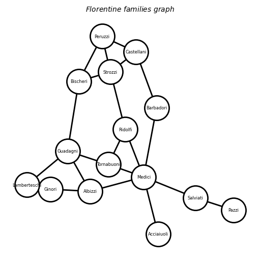
Example: Florenntine families Graph
import networkx as nx
import matplotlib.pyplot as plt

G = nx.florentine_families_graph()
pos = nx.spring_layout(G, iterations=50, seed=0)

fig, axs = plt.subplots(figsize=(5, 5), facecolor='w', constrained_layout=True)

nx.draw_networkx_nodes(G, pos, node_color='white', linewidths=2, edgecolors='k', ax=axs, node_size=1200)
nx.draw_networkx_edges(G, pos, width=2, ax=axs)
nx.draw_networkx_labels(G, pos, font_size=6, ax=axs)

axs.axis('off')
axs.set_title("$Florentine\ families\ graph$", fontsize=10)
Text(0.5, 1.0, '$Florentine\\ families\\ graph$')
Topology measures#
Network size (\(N_i\))#
Number of nodes.
network_size = G.number_of_nodes()
network_size
15
Number of links (\(E_i\))#
Number of edges or connections.
number_of_links = G.number_of_edges()
number_of_links
20
Node degree (\(K_{i,u}\))#
G.degree()
DegreeView({'Acciaiuoli': 1, 'Medici': 6, 'Castellani': 3, 'Peruzzi': 3, 'Strozzi': 4, 'Barbadori': 2, 'Ridolfi': 3, 'Tornabuoni': 3, 'Albizzi': 3, 'Salviati': 2, 'Pazzi': 1, 'Bischeri': 3, 'Guadagni': 4, 'Ginori': 1, 'Lamberteschi': 1})
G.degree()
DegreeView({'Acciaiuoli': 1, 'Medici': 6, 'Castellani': 3, 'Peruzzi': 3, 'Strozzi': 4, 'Barbadori': 2, 'Ridolfi': 3, 'Tornabuoni': 3, 'Albizzi': 3, 'Salviati': 2, 'Pazzi': 1, 'Bischeri': 3, 'Guadagni': 4, 'Ginori': 1, 'Lamberteschi': 1})
dict(G.degree()).values()
dict_values([1, 6, 3, 3, 4, 2, 3, 3, 3, 2, 1, 3, 4, 1, 1])
G_degrees = np.array(list(dict(G.degree()).values()))
G_degrees
array([1, 6, 3, 3, 4, 2, 3, 3, 3, 2, 1, 3, 4, 1, 1])
Density (\(d_i\))#
Ratio of actual connections \(d_i = \frac{2 E_i}{N_i (N_i - 1)}\) for undirected graphs and \(d_i = \frac{E_i}{N_i (N_i - 1)}\) for directed ones.
density = nx.density(G)
density, 2*(number_of_links/(network_size*(network_size-1)))
(0.19047619047619047, 0.19047619047619047)
Accumulated degree (\(K_i\))#
Total contacts in Graph \(i\).
\(K_i = \sum_n k_n\)
accumulated_degree = np.sum(G_degrees)
accumulated_degree
40
Number of components (\(c_i\))#
number_connected_components = nx.number_connected_components(G)
number_connected_components
1
Network structure/fragmentation.
Mean clustering coefficient \(\langle C_i \rangle\)#
Probabbility of common neighbours.
\(\langle C_i \rangle = \frac{1}{N_i} \sum_n C^\prime_{n,i}\), where \(C^\prime_{n,i} = \frac{E^{(n)}}{k_n(k_n-1)}\)
mean_clustering_coef = nx.average_clustering(G)
mean_clustering_coef
0.16
Number of triangles (\(\#\Delta\))#
Number of triangles that includes a given node as one of its vertex.
nx.triangles(G)
{'Acciaiuoli': 0,
 'Medici': 1,
 'Castellani': 1,
 'Peruzzi': 2,
 'Strozzi': 2,
 'Barbadori': 0,
 'Ridolfi': 1,
 'Tornabuoni': 1,
 'Albizzi': 0,
 'Salviati': 0,
 'Pazzi': 0,
 'Bischeri': 1,
 'Guadagni': 0,
 'Ginori': 0,
 'Lamberteschi': 0}
G_tri = np.array(list(dict(nx.triangles(G)).values()))
G_tri
array([0, 1, 1, 2, 2, 0, 1, 1, 0, 0, 0, 1, 0, 0, 0])
average_triangles = np.mean(G_tri)
average_triangles
0.6
Average path length \(\langle l \rangle\)#
Social accessibility between non-interactings.
\(\langle l \rangle = \sum \sum l_{i,j}\)
average_shortest_path_length = nx.average_shortest_path_length(G)
average_shortest_path_length
2.4857142857142858
Example: Comparison of topology metric between two networks#
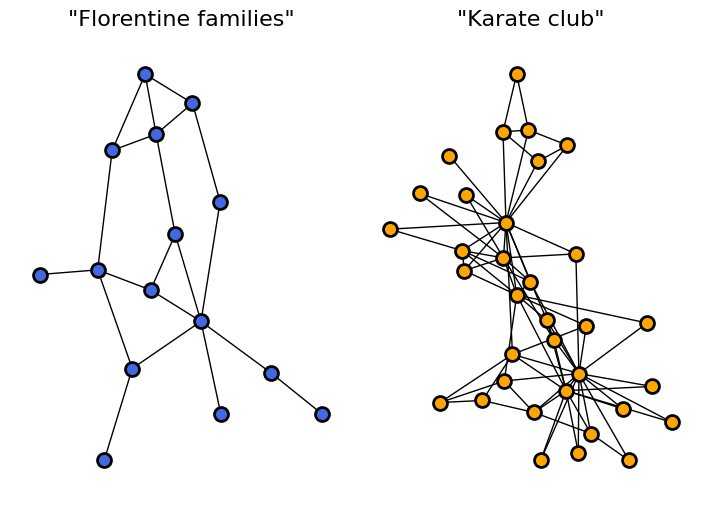
In this section, we will compare the topology of two networks based on some of previous measures.
G1 = nx.florentine_families_graph()
G2 = nx.karate_club_graph()
fig, axs = plt.subplots(figsize=(7,5), facecolor='w', nrows=1, ncols=2, constrained_layout=True) #, gridspec_kw={'width_ratios': [1.5, 1]})

pos = nx.spring_layout(G1, iterations=100, seed=0)
sc = nx.draw_networkx_nodes(G1, pos, node_color='royalblue', linewidths=2, edgecolors='k', ax=axs[0], node_size=100)
nx.draw_networkx_edges(G1, pos, width=1, ax=axs[0])

pos = nx.spring_layout(G2, iterations=100, seed=0)
sc = nx.draw_networkx_nodes(G2, pos, node_color='orange', linewidths=2, edgecolors='k', ax=axs[1], node_size=100)
nx.draw_networkx_edges(G2, pos, width=1, ax=axs[1])
axs[0].axis('off'); axs[1].axis('off');
axs[0].set_title('"Florentine families"', fontsize=16)
axs[1].set_title('"Karate club"', fontsize=16)
Text(0.5, 1.0, '"Karate club"')
Thus, for both graphs, we will compute the next metrics:
Network size (\(N_i\))
Number of links (\(E_i\))
Average node degree (\(\langle K_{i} \rangle\))
Density (\(d_i\))
Accumulated degree (\(K_i\))
Mean clustering coefficient (\(\langle C_i \rangle\))
Average number of triangles (\(\langle \# \Delta \rangle\))
Average path length (\(\langle l \rangle\))
def get_topology_values(G):
  # input:
  # G: Networkx Graph
  # out:
  # dict (key: metric name, value: metric value)

  d_topology_vals = {
      "network_size" : G.number_of_nodes(),
      "number_of_links" : G.number_of_edges(),
      "avg_degree" : np.mean(list(dict(G.degree()).values())),
      "density" : nx.density(G),
      "accumulated_degeree" : np.sum(list(dict(G.degree()).values())),
      "avg_clustering_coef" : nx.average_clustering(G),
      "avg_triangles" : np.mean(list(nx.triangles(G).values())),
      "avg_path_length" : nx.average_shortest_path_length(G),
  }

  return d_topology_vals
topology_G1 = get_topology_values(G1)
topology_G2 = get_topology_values(G2)
df = pd.DataFrame([topology_G1, topology_G2], index=["G_1", "G_2"])
df.T
| G_1 | G_2 | |
|---|---|---|
| network_size | 15.000000 | 34.000000 |
| number_of_links | 20.000000 | 78.000000 |
| avg_degree | 2.666667 | 4.588235 |
| density | 0.190476 | 0.139037 |
| accumulated_degeree | 40.000000 | 156.000000 |
| avg_clustering_coef | 0.160000 | 0.570638 |
| avg_triangles | 0.600000 | 3.970588 |
| avg_path_length | 2.485714 | 2.408200 |
References#
Maarten van Steen (2010). Graph Theory and Complex Networks. An Introduction (Book).
Newman, M. (2010). Networks: An Introduction (Book). Robin J. Wilson (1996). Introduction to Graph Theory (eBook: https://www.maths.ed.ac.uk/~v1ranick/papers/wilsongraph.pdf).
Samaniego, H., Franco-Cisterna, M., & Sotomayor-Gómez, B. (2020). The topology of communicating across cities of increasing sizes, or the complex task of “reaching out” in larger cities. Theories and Models of Urbanization: Geography, Economics and Computing Sciences, 97-118. (Article, https://link.springer.com/chapter/10.1007/978-3-030-36656-8_6)