تحلیل مؤلفههای اصلی، بخش 2
از مبانی ریاضی تا پیادهسازی عملی
تحلیل مؤلفههای اصلی (PCA) تکنیکی بنیادی برای کاهش بُعد است که زیرفضایی بهینه و -بعدی را مییابد که بیشترین واریانس داده را در خود دارد. بنیاد ریاضی آن بر یافتن جهتهای متعامد — موسوم به مؤلفههای اصلی — استوار است که بهترتیب واریانس تصویرشده را بیشینه میکنند.
با ماتریس دادهٔ مرکزشدهٔ ، بردارهای یکهٔ را میجوییم که واریانس دادهٔ تصویرشده را بیشینه کنند:
این بهینهسازی به مسئلهٔ کلیدی مقدار ویژه میانجامد:
که ماتریس کوواریانس است.
در بخشهای بعدی، جواب این مسئله را گامبهگام استنتاج میکنیم و تفسیر هندسی آن را نشان میدهیم.
Source
import numpy as np
import matplotlib.pyplot as plt
from sklearn.decomposition import PCA

# Generate synthetic data with elliptical shape
np.random.seed(42)
n_samples = 100
mean = [0, 0]
cov = [[1, 0.6], [0.6, 0.5]]  # Covariance matrix for elliptical distribution
data = np.random.multivariate_normal(mean, cov, n_samples)

# Center the data
centered_data = data - np.mean(data, axis=0)

# Perform PCA
pca = PCA()
pca.fit(centered_data)
components = pca.components_
explained_variance = pca.explained_variance_ratio_

# Project data onto principal components
projected_data = pca.transform(centered_data)

# Create figure
plt.figure(figsize=(12, 8))

# Plot original data
plt.scatter(centered_data[:, 0], centered_data[:, 1], alpha=0.5, label='Original Data', color='blue')

# Plot principal components as elegant vectors
pc_scale = 2.1  # Scaling factor for PC vectors
plt.quiver(0, 0, components[0,0]*pc_scale, components[0,1]*pc_scale,
          color='lightcoral', scale=1, scale_units='xy', angles='xy', width=0.002,
          label=f'PC1 (Variance: {100*explained_variance[0]:.1f}%)')
plt.quiver(0, 0, components[1,0]*pc_scale, components[1,1]*pc_scale,
          color='lightgreen', scale=1, scale_units='xy', angles='xy', width=0.002,
          label=f'PC2 (Variance: {100*explained_variance[1]:.1f}%)')

# Plot projections onto PC1 (first principal component)
for point in centered_data:
    projection_pc1 = np.dot(point, components[0]) * components[0]
    plt.plot([point[0], projection_pc1[0]], [point[1], projection_pc1[1]],
             'r--', alpha=0.3, linewidth=0.7)

# Plot projections onto PC2 (second principal component)
for point in centered_data:
    projection_pc2 = np.dot(point, components[1]) * components[1]
    plt.plot([point[0], projection_pc2[0]], [point[1], projection_pc2[1]],
             'g--', alpha=0.2, linewidth=0.6)

# Plot the projected points on PC1
projected_pc1 = np.dot(projected_data[:, 0][:, np.newaxis], components[0:1, :])
plt.scatter(projected_pc1[:, 0], projected_pc1[:, 1], color='red', alpha=0.7,
            label='Projections on PC1', s=30)

# Plot the projected points on PC2
projected_pc2 = np.dot(projected_data[:, 1][:, np.newaxis], components[1:2, :])
plt.scatter(projected_pc2[:, 0], projected_pc2[:, 1], color='green', alpha=0.7,
            label='Projections on PC2', s=30)

# Add annotations and legend
plt.axhline(0, color='black', linestyle='--', alpha=0.2)
plt.axvline(0, color='black', linestyle='--', alpha=0.2)
plt.xlabel('Feature 1')
plt.ylabel('Feature 2')
plt.title('PCA: Principal Components and Data Projections\n'
          f'PC1 explains {100*explained_variance[0]:.1f}% of variance\n'
          f'PC2 explains {100*explained_variance[1]:.1f}% of variance')
plt.legend(loc="lower right")
plt.grid(alpha=0.2)
plt.axis('equal')
plt.show()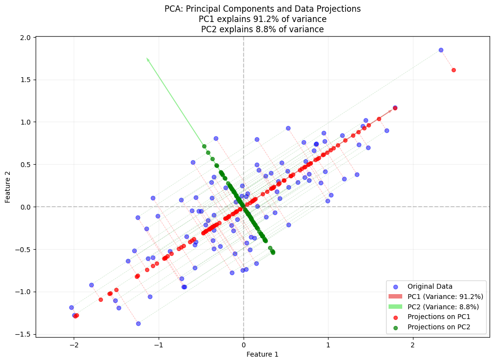
مبانی جبر خطی
نمایش ماتریس داده
ماتریس دادهٔ با سطر (نمونه) و ستون (ویژگی) را میتوان چنین نوشت:
هر سطر یک نمونه در فضای -بعدی را نشان میدهد.
Source
import numpy as np
import matplotlib.pyplot as plt
from sklearn.datasets import load_iris, make_blobs
from sklearn.decomposition import PCA
import seaborn as sns

# Set style for better plots
plt.style.use('seaborn-v0_8')
np.random.seed(42)# Example: Vector operations
a = np.array([3, 4])
b = np.array([1, 2])
# Dot product
dot_product = np.dot(a, b)
print(f"Dot product: {dot_product}")
# Vector norms
norm_a = np.linalg.norm(a)
norm_b = np.linalg.norm(b)
print(f"Norm of a: {norm_a:.2f}")
print(f"Norm of b: {norm_b:.2f}")
# Angle between vectors
cos_theta = dot_product / (norm_a * norm_b)
theta_rad = np.arccos(cos_theta)
theta_deg = np.degrees(theta_rad)
print(f"Angle between vectors: {theta_deg:.2f} degrees")Dot product: 11
Norm of a: 5.00
Norm of b: 2.24
Angle between vectors: 10.30 degrees
تصویر بردارها (استنتاج و شهود هندسی)
استنتاج فرمول تصویر
با عملیات پایهٔ برداری شروع میکنیم تا فرمول تصویر را طبیعتاً استنتاج کنیم:
رابطهٔ ضرب داخلی و زاویه: از تعریفهای پیشین میدانیم:
این همراستایی میان بردارها را میسنجد.
تصویر اسکالر (طول سایه): طول سایهٔ روی چنین است:
برای بردارهای یکه این ساده میشود به .
تصویر برداری: برای رسیدن به شکل برداری، تصویر اسکالر را در بردار یکهٔ ضرب میکنیم:
فرمول نهایی تصویر
نکتههای کلیدی:
تفسیر ضرب داخلی:
صورت همراستایی را میسنجد
مخرج برای طول بردار نرمالسازی میکند
حالت خاص — بردار یکه: وقتی :
معنای هندسی:
سایهٔ روی است
باقیماندهٔ بر عمود است
مثال
بگذارید و .
گام 1: .
گام 2: .
گام 3: تصویر .
مؤلفهٔ عمود: .
تفسیر: چون در راستای محور x است، فقط مؤلفهٔ x از را نگه میدارد و مؤلفهٔ باقیماندهٔ y را میگیرد که بر عمود است.
پیوند با PCA: این مفهوم تصویر، قلب هندسی PCA است. در بخش بعد آن را به چند بُعد گسترش میدهیم و به جواب PCA از راه تجزیهٔ مقادیر ویژه میرسیم.
# Example: Vector projection
def project_vector(b, a):
    """Project vector b onto vector a"""
    projection = (np.dot(a, b) / np.dot(a, a)) * a
    perpendicular = b - projection
    return projection, perpendicular

# Example vectors
a = np.array([1, 0])  # Direction vector
b = np.array([3, 2])  # Vector to project

b_parallel, b_perp = project_vector(b, a)

print(f"Original vector b: {b}")
print(f"Projection onto a: {b_parallel}")
print(f"Perpendicular component: {b_perp}")
print(f"Verification (should equal b): {b_parallel + b_perp}")
Original vector b: [3 2]
Projection onto a: [3. 0.]
Perpendicular component: [0. 2.]
Verification (should equal b): [3. 2.]
Source
plt.rcParams['font.family'] = 'DejaVu Sans'

# Visualization of vector projection
plt.figure(figsize=(10, 5))

# Plot vectors
plt.quiver(0, 0, a[0], a[1], angles='xy', scale_units='xy', scale=1, color='red', width=0.005, label='Direction vector a')
plt.quiver(0, 0, b[0], b[1], angles='xy', scale_units='xy', scale=1, color='blue', width=0.003, label='Original vector b')
plt.quiver(0, 0, b_parallel[0], b_parallel[1], angles='xy', scale_units='xy', scale=1, color='green', width=0.003, label='Projection b∥')
plt.quiver(b_parallel[0], b_parallel[1], b_perp[0], b_perp[1], angles='xy', scale_units='xy', scale=1, color='orange', width=0.003, label='Perpendicular b⊥')

# Add dotted line to show projection
plt.plot([b[0], b_parallel[0]], [b[1], b_parallel[1]], 'k--', alpha=0.5)

# Set axis limits with some padding
padding = 0.5
plt.xlim(min(0, b[0], b_parallel[0]) - padding, max(a[0], b[0], b_parallel[0]) + padding)
plt.ylim(min(0, b[1], b_parallel[1]) - padding, max(a[1], b[1], b_parallel[1]) + padding)
# plt.xlim(-0.5, 3.5)
# plt.ylim(-0.5, 2.5)
plt.grid(True, alpha=0.3)
plt.axis('equal')
plt.legend()
plt.title('Vector Projection Demonstration')
plt.xlabel('X')
plt.ylabel('Y')
plt.show()

# Print the vectors and their magnitudes
print(f"Vector a: {a}, magnitude: {np.linalg.norm(a):.2f}")
print(f"Vector b: {b}, magnitude: {np.linalg.norm(b):.2f}")
print(f"b_parallel: {b_parallel}, magnitude: {np.linalg.norm(b_parallel):.2f}")
print(f"b_perpendicular: {b_perp}, magnitude: {np.linalg.norm(b_perp):.2f}")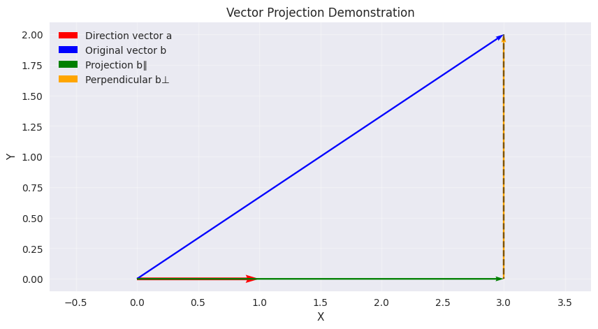
Vector a: [1 0], magnitude: 1.00
Vector b: [3 2], magnitude: 3.61
b_parallel: [3. 0.], magnitude: 3.00
b_perpendicular: [0. 2.], magnitude: 2.00
تبدیل پایه
تغییر پایه
هر بردار را میتوان برحسب یک پایهٔ متعامد یکهٔ تازه نوشت:
که بردارهای پایهٔ تازه را در ستونهایش دارد و مختصات در پایهٔ تازه است:
این کار میکند چون متعامد یکه بودن میدهد، پس مختصات در راستای بهسادگی ضرب داخلی است.
# Example: Basis transformation
# Original vector
x = np.array([0.5, 1, 2])

# Standard basis (i, j, k)
standard_basis = np.eye(3)
i = standard_basis[:, 0]
j = standard_basis[:, 1]
k = standard_basis[:, 2]

print(f"Original vector x: {x}")
print(f"In standard basis: {x[0]}i + {x[1]}j + {x[2]}k")

# Create a new orthonormal basis (rotated 45° in xy-plane)
u1 = np.array([1/np.sqrt(2), 1/np.sqrt(2), 0])
u2 = np.array([-1/np.sqrt(2), 1/np.sqrt(2), 0])
u3 = np.array([0, 0, 1])

# New basis matrix
U = np.column_stack([u1, u2, u3])
print(U)
Original vector x: [0.5 1. 2. ]
In standard basis: 0.5i + 1.0j + 2.0k
[[ 0.70710678 -0.70710678 0. ]
[ 0.70710678 0.70710678 0. ]
[ 0. 0. 1. ]]
Source
# Create 3D plot
fig = plt.figure(figsize=(15, 5))

# Plot 1: Original vector and standard basis
ax1 = fig.add_subplot(121, projection='3d')
ax1.set_title('Original Vector and Standard Basis')

# Plot standard basis vectors
ax1.quiver(0, 0, 0, i[0], i[1], i[2], color='r', label='i')
ax1.quiver(0, 0, 0, j[0], j[1], j[2], color='g', label='j')
ax1.quiver(0, 0, 0, k[0], k[1], k[2], color='b', label='k')

# Plot original vector
ax1.quiver(0, 0, 0, x[0], x[1], x[2], color='purple', label='x')

# Plot xy-plane for reference
xx, yy = np.meshgrid(range(-2, 3), range(-2, 3))
zz = np.zeros_like(xx)
ax1.plot_surface(xx, yy, zz, alpha=0.1, color='gray')

# Plot 2: Rotated basis and transformed vector
ax2 = fig.add_subplot(122, projection='3d')
ax2.set_title('Rotated Basis and Transformed Vector')

# Plot rotated basis vectors
ax2.quiver(0, 0, 0, u1[0], u1[1], u1[2], color='r', label='u1')
ax2.quiver(0, 0, 0, u2[0], u2[1], u2[2], color='g', label='u2')
ax2.quiver(0, 0, 0, u3[0], u3[1], u3[2], color='b', label='u3')

# Plot original vector
ax2.quiver(0, 0, 0, x[0], x[1], x[2], color='purple', label='x')

# Plot rotated xy-plane
R = np.array([[1/np.sqrt(2), -1/np.sqrt(2), 0],
              [1/np.sqrt(2), 1/np.sqrt(2), 0],
              [0, 0, 1]])
rotated_points = R @ np.array([xx.flatten(), yy.flatten(), zz.flatten()])
rotated_xx = rotated_points[0].reshape(xx.shape)
rotated_yy = rotated_points[1].reshape(yy.shape)
rotated_zz = rotated_points[2].reshape(zz.shape)
ax2.plot_surface(rotated_xx, rotated_yy, rotated_zz, alpha=0.1, color='gray')

# Set equal aspects and labels
for ax in [ax1, ax2]:
    ax.set_xlabel('X')
    ax.set_ylabel('Y')
    ax.set_zlabel('Z')
    ax.set_xlim([-2, 2])
    ax.set_ylim([-2, 2])
    ax.set_zlim([-2, 2])
    # ax.set_xticks([])  # Disable x-axis numbers
    ax.set_yticks([])  # Disable y-axis numbers
    ax.set_zticks([])  # Disable z-axis numbers
    ax.legend()

plt.tight_layout()
plt.show()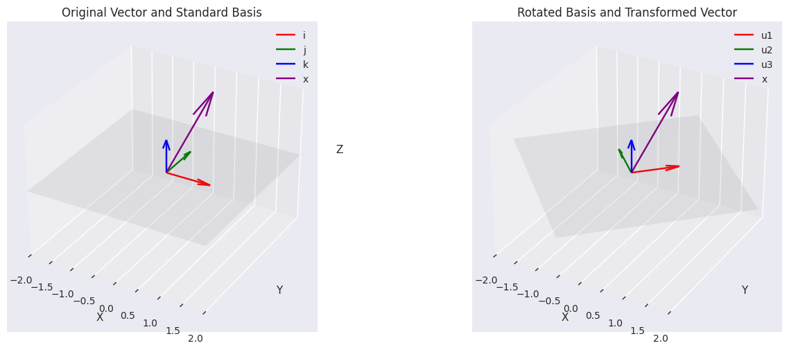
بنیاد ریاضی ماتریس دوران
مبانی دوران در دو بعد
ماتریس دوران بردارها را با چرخاندنشان به اندازهٔ زاویهٔ مشخص θ دگرگون میکند و طولشان را نگه میدارد. برای دورانی 45 درجه در صفحهٔ xy (θ = π/4 رادیان)، ماتریس دوران پایه چنین است:
برای θ = 45 درجه:
پس ماتریس دوران 45 درجه چنین میشود:
تبدیل پایه
در کد پیشین، این ماتریس دوران بردارهای پایهٔ تازهای تعریف میکند:
u1 = np.array([1/np.sqrt(2), 1/np.sqrt(2), 0])  # Rotated x-axis
u2 = np.array([-1/np.sqrt(2), 1/np.sqrt(2), 0]) # Rotated y-axis
u3 = np.array([0, 0, 1]) # Unchanged z-axisاینها پایهای متعامد یکه میسازند:
: محور x اصلی که 45 درجه پادساعتگرد چرخیده
: محور y اصلی که 45 درجه پادساعتگرد چرخیده
: محور z اصلی (بدون تغییر)
ویژگیهای کلیدی
متعامد یکه بودن:
دترمینان: (جهتگیری را حفظ میکند)
وارون: (ترانهاده دوران را برمیگرداند)
دگرگونی بردار
برای هر بردار ، نسخهٔ چرخیده چنین است:
این با رویکرد تبدیل پایهٔ ما میخواند که در آن:
چرا کار میکند
ستونهای دقیقاً تصویر بردارهای پایهٔ استاندارد زیر دوراناند. وقتی ضرب میکنیم:
پس دقیقاً میگوید هر محور کجا میرود — و همین دلیل است که ستونهایش پایهٔ تازه را میسازند.
# Transform to new basis
a = U.T @ x

print(f"\nIn new basis: {a[0]:.2f}u1 + {a[1]:.2f}u2 + {a[2]:.2f}u3")

# Verify: transform back to original
x_reconstructed = U @ a
print(f"\nReconstructed x: {x_reconstructed}")
print(f"Reconstruction error: {np.linalg.norm(x - x_reconstructed):.10f}")
In new basis: 1.06u1 + 0.35u2 + 2.00u3

Reconstructed x: [0.5 1.  2. ]
Reconstruction error: 0.0000000000
بنیاد ریاضی PCA
مسئلهٔ بیشینهسازی واریانس
PCA پایهای متعامد یکه میجوید که با بهینهسازی متوالی بیشترین واریانس داده را در خود بگیرد:
مؤلفهٔ اصلی اول: بردار یکهٔ را بیاب که واریانس تصویرشده را بیشینه کند:
مؤلفههای بعدی: هر با بیشینه کردن واریانس عمود بر مؤلفههای پیشین یافته میشود:
به کوتاهی، مؤلفهٔ اصلی اول جهت بیشترین پخششدگی داده است. هر مؤلفهٔ بعدی باید بر همهٔ مؤلفههای پیشین عمود باشد تا اطلاعات واقعاً تازه و مستقل بگیرد.
یافتن مؤلفهٔ اصلی اول
بردار یکهٔ را میجوییم که واریانس دادهٔ تصویرشده را بیشینه کند:
که میانگین مقدارهای تصویرشده است (با استفاده از خطیبودن ضرب داخلی).
بسط واریانس:
بگذارید تصویر اسکالر نمونهٔ ام را نشان دهد.
واریانس چنین میشود:
بگذارید نقطههای دادهٔ مرکزشده را نشان دهد. گامبهگام بسط میدهیم:
از اتحاد استفاده کنید و توجه کنید که :
بازآرایی کنید و را میان و بگذارید:
و را از جمع بیرون بکشید:
ماتریس کوواریانس نمونه را بشناسید:
بهطور معادل، با ماتریس دادهٔ مرکزشده :
پس واریانس دادهٔ تصویرشده چنین است:
بهینهسازی مقید با ضریب لاگرانژ
واریانس تصویرشدهٔ را با قید بیشینه میکنیم. با وارد کردن ضریب لاگرانژ ، لاگرانژی چنین است:
جواب
گرادیان نسبت به را صفر میگذاریم:
این دقیقاً معادلهٔ مقدار ویژه است: باید بردار ویژهٔ ماتریس کوواریانس باشد و مقدار ویژهٔ متناظر.
انتخاب مقدار ویژهٔ درست
با جایگذاری در بیان واریانس:
واریانس تصویرشده برابر مقدار ویژهٔ است. برای بیشینه کردن واریانس، پس یعنی بزرگترین مقدار ویژهٔ را برمیگزینیم. بردار ویژهٔ متناظر جهت بیشترین واریانس را تعریف میکند — مؤلفهٔ اصلی اول.
Source
import numpy as np
import matplotlib.pyplot as plt

# Generate synthetic data
np.random.seed(42)
mean = [0, 0]
cov = [[1, 0.6], [0.6, 0.5]]
X = np.random.multivariate_normal(mean, cov, 100)
# Center the data
X_mean = np.mean(X, axis=0)
Z = X - X_mean
# Compute covariance matrix
cov_matrix = np.dot(Z.T, Z) / (len(Z) - 1)
# Compute eigenvalues and eigenvectors
eigenvalues, eigenvectors = np.linalg.eigh(cov_matrix)
# Sort by descending eigenvalues
idx = eigenvalues.argsort()[::-1]
eigenvalues = eigenvalues[idx]
eigenvectors = eigenvectors[:, idx]
# Extract PC1 (first principal component)
u1 = eigenvectors[:, 0]
λ1 = eigenvalues[0]
print(f"u1 = {u1}, λ1 = {λ1:.2f}")u1 = [-0.83818843 -0.54538075], λ1 = 1.03
Source
# Create figure
plt.figure(figsize=(8, 6))

# Plot original centered data
plt.scatter(Z[:, 0], Z[:, 1], alpha=0.9, label='Original Data (Centered)')

# Plot PC1 direction (scaled by standard deviation)
plt.quiver(0, 0, u1[0]*2*np.sqrt(λ1), u1[1]*2*np.sqrt(λ1),
           color='green', scale=1, scale_units='xy', angles='xy', width=0.007,
           label=f'PC1 (λ={λ1:.2f})')

# Project data onto PC1
projections = np.outer(Z @ u1, u1)  # Projection vectors

# Plot projections
plt.scatter(projections[:, 0], projections[:, 1], color='red', alpha=0.7,
           s=30, label='Projections on PC1')

# Draw projection lines
for point, proj in zip(Z, projections):
    plt.plot([point[0], proj[0]], [point[1], proj[1]],
             'r--', alpha=0.3, linewidth=0.7)

# Formatting
plt.axhline(0, color='black', linestyle='--', alpha=0.2)
plt.axvline(0, color='black', linestyle='--', alpha=0.2)
plt.title('First Principal Component and Projections\n(Maximum Variance Direction)')
plt.xlabel('Feature 1')
plt.ylabel('Feature 2')
plt.legend()
plt.grid(alpha=0.2)
plt.axis('equal')
plt.tight_layout()
plt.show()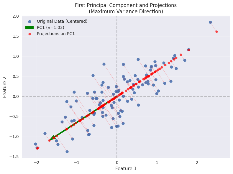
الگوریتم PCA
با ماتریس دادهٔ :
داده را مرکز کن:
ماتریس کوواریانس را حساب کن:
مقادیر و بردارهای ویژهٔ را حساب کن
مقادیر ویژه را به ترتیب نزولی مرتب کن
بردار ویژهٔ اول را بهعنوان مؤلفههای اصلی انتخاب کن
داده را تصویر کن:
def pca_from_scratch(X, n_components):
    """
    Implement PCA from scratch

    Parameters:
    X: data matrix (n_samples, n_features)
    n_components: number of principal components to keep

    Returns:
    X_transformed: transformed data
    components: principal components
    eigenvalues: eigenvalues
    mean: data mean
    """
    # Step 1: Center the data
    X_mean = np.mean(X, axis=0)
    Z = X - X_mean

    # Step 2: Compute covariance matrix
    n_samples = X.shape[0]
    cov_matrix = np.dot(Z.T, Z) / (n_samples - 1)

    # Step 3: Compute eigenvalues and eigenvectors
    eigenvalues, eigenvectors = np.linalg.eigh(cov_matrix)

    # Step 4: Sort eigenvalues and eigenvectors in descending order
    idx = eigenvalues.argsort()[::-1]
    eigenvalues = eigenvalues[idx]
    eigenvectors = eigenvectors[:, idx]

    # Step 5: Select top n_components
    components = eigenvectors[:, :n_components]

    # Step 6: Project the data
    X_transformed = np.dot(Z, components)

    return X_transformed, components, eigenvalues, X_mean

def reconstruct_data(X_transformed, components, mean):
    """Reconstruct original data from PCA representation"""
    X_reconstructed = np.dot(X_transformed, components.T) + mean
return X_reconstructedگردشکار PCA: از یک نمونه تا کل ماتریس
تصویر و بازسازی (یک نقطهٔ داده)
گام 1: مرکز کردن با میانگین
با بردار دادهٔ خام:
بردار میانگین را کم کنید:
که میانگین همهٔ نمونهها است.
گام 2: تصویر (کاهش بُعد)
را روی مؤلفهٔ اصلی اول تصویر کنید: (اسکالر، تصویر روی )
نمایش کاهشیافته (در فضای PCA) چنین است:
گام 3: بازسازی (تقریب)
دادهٔ مرکزشده را با مؤلفههای اصلی بازسازی کنید:
میانگین را برگردانید تا به فضای اصلی برگردید:
تفسیر هندسی
بازسازی نزدیکترین تقریب با فقط جهت است.
خطای از کنار گذاشتن مؤلفههای اصلی باقیمانده میآید.
تعمیم به کل ماتریس داده
گام 1: مرکز کردن با میانگین (شکل ماتریسی)
ماتریس دادهٔ اصلی:
دادهٔ مرکزشده:
که برداری ستونی از یکها است.
گام 2: تصویر (تبدیل PCA)
همهٔ نمونهها را روی مؤلفهٔ اصلی اول تصویر کنید ():
هر سطر نمایش کاهشیافتهٔ یک نمونه را دارد.
گام 3: بازسازی (شکل ماتریسی)
دادهٔ مرکزشده را بازسازی کنید:
= ستون ام (امتیازهای مؤلفهٔ اصلی ).
هر جملهٔ ماتریسی رتبه-1 است.
برگشت به فضای اصلی:
پیوند با پیادهسازی پایتون
تصویر (کاهش بُعد)
X_transformed = Z @ U_r # ≡ Z U_r (n × r matrix)بازسازی
Z_recon = X_transformed @ U_r.T  # ≡ A U_r^T (n × d)
X_recon = Z_recon + mean # Add back meanنکتههای کلیدی
از یک نمونه تا کل ماتریس:
با یک بردار تنها شروع کنید تا تصویر/بازسازی را بفهمید.
با عملیات ماتریسی به کل مجموعهداده تعمیم دهید.
فشردهسازی با اتلاف:
نگه داشتن فقط مؤلفهٔ اصلی یعنی بازسازی تقریبی است.
خطا به مقادیر ویژهٔ کنارگذاشته بستگی دارد.
PCA بهعنوان دوران:
تصویر = چرخاندن داده برای همراستا شدن با جهتهای بیشترین واریانس.
بازسازی = چرخاندن برگشتی، با استفاده از مهمترین جهتها.
همارزی دو نگاه بهینهسازی در PCA و تحلیل خطا (مطالعهٔ بیشتر)
PCA را میتوان از دو نگاه همارز استنتاج کرد:
بیشینهسازی واریانس: یافتن جهتهایی که واریانس تصویرشده را بیشینه میکنند.
کمینهسازی خطای بازسازی: یافتن جهتهایی که میانگین مربع خطای بازسازی را کمینه میکنند.
همارزی آنها را ریاضی اثبات میکنیم و خطا را تحلیل میکنیم.
1. صورت بیشینهسازی واریانس
هدف: یافتن بردار یکهٔ که واریانس دادهٔ تصویرشده را بیشینه کند:
جواب، بردار ویژهٔ با بزرگترین مقدار ویژه است.
2. کمینهسازی خطای بازسازی
هدف: یافتن که MSE میان دادهٔ اصلی و بازسازیاش را کمینه کند:
3. اثبات همارزی
خطای بازسازی را بسط دهید:
پس MSE چنین میشود:
مشاهدات کلیدی:
جملهٔ ثابت است (واریانس کل داده).
کمینه کردن MSE همارز بیشینه کردن (واریانس تصویرشده) است.
4. تحلیل خطا در PCA
مؤلفههای تصویر و باقیمانده
برای نقطهٔ دادهٔ (مرکزشده) و بازسازیاش با مؤلفهٔ اصلی:
بردار خطا: .
استنتاج میانگین مربع خطا (MSE)
کل MSE روی همهٔ نمونهها چنین است:
پیوند با مقادیر ویژه
طبق تعریف، واریانس در راستای چنین است:
پس:
5. نتیجه و جمعبندی
دو صورت همارز: بیشینهسازی واریانس و کمینهسازی خطا در PCA همارزند.
تفسیر مقدار ویژه: MSE برابر مجموع مقادیر ویژهٔ کنارگذاشته است، چون:
هر واریانس در راستای مؤلفهٔ اصلی است.
کنار گذاشتن مؤلفههای تا دقیقاً واریانس را از دست میدهد.
بهینگی: جواب PCA همزمان واریانس حفظشده را بیشینه و خطای بازسازی را کمینه میکند.
رابطههای کلیدی:
| مفهوم | فرمول | تفسیر |
|---|---|---|
| تصویر | بازسازی با مؤلفهٔ اصلی اول | |
| خطا | باقیمانده از مؤلفههای کنارگذاشته | |
| MSE | مجموع واریانس مؤلفههای کنارگذاشته |
Source
# Load the Iris dataset
iris = load_iris()
X_iris = iris.data
y_iris = iris.target
feature_names = iris.feature_names

print(f"Original data shape: {X_iris.shape}")
print(f"Features: {feature_names}")

# Apply PCA
X_pca, components, eigenvalues, mean = pca_from_scratch(X_iris, n_components=2)

# Calculate explained variance ratio
total_var = eigenvalues.sum()
explained_var_ratio = eigenvalues[:2] / total_var

print(f"\nExplained variance ratio:")
print(f"PC1: {explained_var_ratio[0]:.3f} ({explained_var_ratio[0]*100:.1f}%)")
print(f"PC2: {explained_var_ratio[1]:.3f} ({explained_var_ratio[1]*100:.1f}%)")
print(f"Total: {explained_var_ratio.sum():.3f} ({explained_var_ratio.sum()*100:.1f}%)")
Original data shape: (150, 4)
Features: ['sepal length (cm)', 'sepal width (cm)', 'petal length (cm)', 'petal width (cm)']
Explained variance ratio:
PC1: 0.925 (92.5%)
PC2: 0.053 (5.3%)
Total: 0.978 (97.8%)
Source
# Visualize the results
plt.figure(figsize=(15, 5))

# Plot 1: Original data (first two features)
plt.subplot(1, 3, 1)
scatter = plt.scatter(X_iris[:, 0], X_iris[:, 1], c=y_iris, cmap='viridis')
plt.xlabel(feature_names[0])
plt.ylabel(feature_names[1])
plt.title('Original Data (First 2 Features)')
plt.colorbar(scatter)

# Plot 2: PCA transformed data
plt.subplot(1, 3, 2)
scatter = plt.scatter(X_pca[:, 0], X_pca[:, 1], c=y_iris, cmap='viridis')
plt.xlabel('First Principal Component')
plt.ylabel('Second Principal Component')
plt.title('PCA Transformed Data')
plt.colorbar(scatter)

# Plot 3: Explained variance
plt.subplot(1, 3, 3)
plt.bar(['PC1', 'PC2', 'PC3', 'PC4'], eigenvalues/total_var * 100)
plt.ylabel('Explained Variance Ratio (%)')
plt.title('Explained Variance by Components')
plt.xticks(rotation=45)

plt.tight_layout()
plt.show()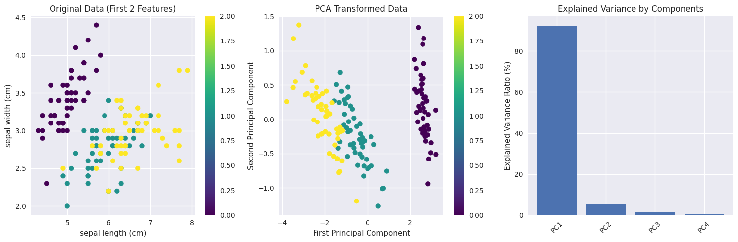
تحلیل خطای بازسازی
Source
# Analyze reconstruction error for different numbers of components
n_features = X_iris.shape[1]
reconstruction_errors = []

for n_comp in range(1, n_features + 1):
    X_pca_temp, components_temp, _, mean_temp = pca_from_scratch(X_iris, n_comp)
    X_reconstructed = reconstruct_data(X_pca_temp, components_temp, mean_temp)

    # Calculate mean squared error
    mse = np.mean((X_iris - X_reconstructed) ** 2)
    reconstruction_errors.append(mse)

plt.figure(figsize=(10, 6))
plt.plot(range(1, n_features + 1), reconstruction_errors, 'bo-')
plt.xlabel('Number of Principal Components')
plt.ylabel('Mean Squared Reconstruction Error')
plt.title('Reconstruction Error vs Number of Components')
plt.grid(True, alpha=0.3)
plt.xticks(range(1, n_features + 1))

for i, error in enumerate(reconstruction_errors):
    plt.annotate(f'{error:.4f}', (i+1, error), textcoords="offset points", xytext=(0,10), ha='center')

plt.show()

print("Reconstruction errors:")
for i, error in enumerate(reconstruction_errors):
    print(f"{i+1} components: MSE = {error:.6f}")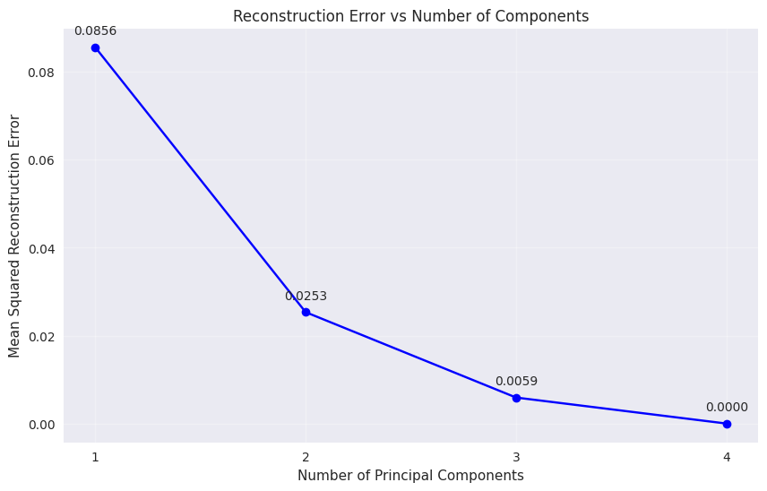
Reconstruction errors:
1 components: MSE = 0.085604
2 components: MSE = 0.025341
3 components: MSE = 0.005919
4 components: MSE = 0.000000
مثال دادهٔ با ابعاد بالا
Source
# Generate high-dimensional data with intrinsic low-dimensional structure
np.random.seed(42)
n_samples = 200
n_features = 50
n_informative = 3  # True dimensionality

# Generate data with only 3 informative dimensions
X_high_dim = np.random.randn(n_samples, n_informative)

# Create a random mixing matrix to embed in high-dimensional space
mixing_matrix = np.random.randn(n_informative, n_features)
X_mixed = X_high_dim @ mixing_matrix

# Add some noise
noise_level = 0.1
X_noisy = X_mixed + noise_level * np.random.randn(n_samples, n_features)

print(f"Generated data shape: {X_noisy.shape}")
print(f"True intrinsic dimensionality: {n_informative}")

# Apply PCA
X_pca_high, components_high, eigenvalues_high, mean_high = pca_from_scratch(X_noisy, n_components=10)

# Calculate cumulative explained variance
total_var_high = eigenvalues_high.sum()
explained_var_ratio_high = eigenvalues_high / total_var_high
cumulative_var = np.cumsum(explained_var_ratio_high)

print(f"\nExplained variance by first 10 components:")
for i in range(10):
    print(f"PC{i+1}: {explained_var_ratio_high[i]:.3f} (cumulative: {cumulative_var[i]:.3f})")
Generated data shape: (200, 50)
True intrinsic dimensionality: 3
Explained variance by first 10 components:
PC1: 0.420 (cumulative: 0.420)
PC2: 0.342 (cumulative: 0.763)
PC3: 0.234 (cumulative: 0.997)
PC4: 0.000 (cumulative: 0.997)
PC5: 0.000 (cumulative: 0.997)
PC6: 0.000 (cumulative: 0.997)
PC7: 0.000 (cumulative: 0.997)
PC8: 0.000 (cumulative: 0.998)
PC9: 0.000 (cumulative: 0.998)
PC10: 0.000 (cumulative: 0.998)
Source
# Visualize the explained variance
plt.figure(figsize=(12, 5))

# Plot 1: Individual explained variance
plt.subplot(1, 2, 1)
plt.bar(range(1, 11), explained_var_ratio_high[:10] * 100)
plt.xlabel('Principal Component')
plt.ylabel('Explained Variance Ratio (%)')
plt.title('Individual Explained Variance')
plt.xticks(range(1, 11))

# Plot 2: Cumulative explained variance
plt.subplot(1, 2, 2)
plt.plot(range(1, 11), cumulative_var[:10] * 100, 'bo-')
plt.axhline(y=95, color='r', linestyle='--', label='95% threshold')
plt.xlabel('Number of Components')
plt.ylabel('Cumulative Explained Variance (%)')
plt.title('Cumulative Explained Variance')
plt.legend()
plt.grid(True, alpha=0.3)
plt.xticks(range(1, 11))

plt.tight_layout()
plt.show()

# Find number of components for 95% variance
n_components_95 = np.argmax(cumulative_var >= 0.95) + 1
print(f"\nNumber of components needed for 95% variance: {n_components_95}")
print(f"This is close to the true intrinsic dimensionality of {n_informative}")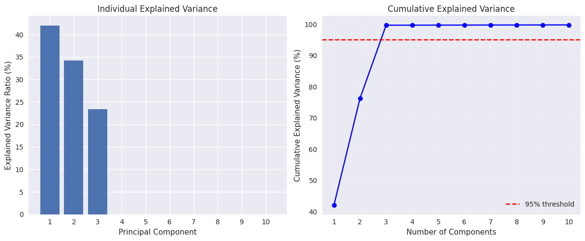
Number of components needed for 95% variance: 3
This is close to the true intrinsic dimensionality of 3
مقایسه با Scikit-learn
Source
# Compare our implementation with scikit-learn
from sklearn.decomposition import PCA as SklearnPCA

# Our implementation
X_pca_ours, components_ours, eigenvalues_ours, mean_ours = pca_from_scratch(X_iris, n_components=2)

# Scikit-learn implementation
pca_sklearn = SklearnPCA(n_components=2)
X_pca_sklearn = pca_sklearn.fit_transform(X_iris)

print("Comparison of implementations:")
print(f"Our explained variance ratio: {eigenvalues_ours[:2]/eigenvalues_ours.sum()}")
print(f"Sklearn explained variance ratio: {pca_sklearn.explained_variance_ratio_}")

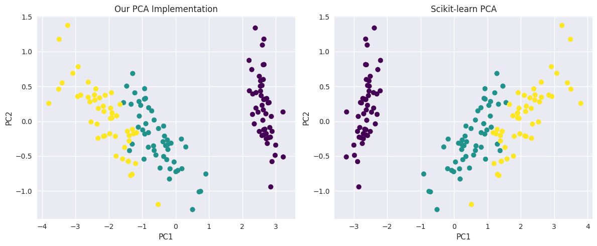
# The signs of eigenvectors might be different, but the results should be equivalent
print(f"\nMean absolute difference in transformed data: {np.mean(np.abs(np.abs(X_pca_ours) - np.abs(X_pca_sklearn))):.10f}")

# Visualize both results
plt.figure(figsize=(12, 5))

plt.subplot(1, 2, 1)
plt.scatter(X_pca_ours[:, 0], X_pca_ours[:, 1], c=y_iris, cmap='viridis')
plt.title('Our PCA Implementation')
plt.xlabel('PC1')
plt.ylabel('PC2')

plt.subplot(1, 2, 2)
plt.scatter(X_pca_sklearn[:, 0], X_pca_sklearn[:, 1], c=y_iris, cmap='viridis')
plt.title('Scikit-learn PCA')
plt.xlabel('PC1')
plt.ylabel('PC2')

plt.tight_layout()
plt.show()
Comparison of implementations:
Our explained variance ratio: [0.92461872 0.05306648]
Sklearn explained variance ratio: [0.92461872 0.05306648]
Mean absolute difference in transformed data: 0.0000000000
بخشی از مقالههای پیشین من دربارهٔ PCA هستند، از جمله Amintoosi & Farbiz (2022)Fathy et al. (2008)Amintoosi et al. (2007)Amintoosi & Poursadeghi (1394)
جمعبندی
این درسنامه پوشش داد:
مبانی جبر خطی: عملیات برداری، نُرمها و زاویهها
تصویر بردارها: بنیاد ریاضی کاهش بُعد
تبدیل پایه: چگونه داده را در دستگاههای مختصات مختلف نمایش دهیم
نظریهٔ PCA: بیشینهسازی واریانس و تجزیهٔ مقادیر ویژه
پیادهسازی: الگوریتم گامبهگام PCA از صفر
کاربردها: مثالهای واقعی با مجموعهدادهٔ Iris و دادهٔ با ابعاد بالا
نکتههای کلیدی:
PCA جهتهای بیشترین واریانس در داده را مییابد
مؤلفههای اصلی بردارهای ویژهٔ ماتریس کوواریانساند
مقادیر ویژه مقدار واریانس گرفتهشده توسط هر مؤلفه را نشان میدهند
PCA از نظر خطای بازسازی، کاهش بُعد خطی بهینه میدهد
تعداد مؤلفهها را میتوان بر پایهٔ آستانهٔ واریانس توضیحدادهشدهٔ مطلوب برگزید
تمرینها
ماتریس تصویر روی پوشش یک بردار یکهٔ را استنتاج کنید و نشان دهید متقارن و خودتوان است.
نشان دهید پس از تغییر پایه با یک متعامد، ماتریس کوواریانس میشود، و توضیح دهید چرا این پایهٔ ویژه را خاص میکند.
PCA را با بیشینه کردن با قید استنتاج کنید و ضریب لاگرانژ را با واریانس حفظشده شناسایی کنید.
- Amintoosi, M., & Farbiz, F. (2022). Eigenbackground Revisited: Can We Model the Background with Eigenvectors? Journal of Mathematical Imaging and Vision, 64(5), 463–477.
- Fathy, M., Mozayani, N., & Amintoosi, M. (2008). Outlier Removal for Super-Resolution Problem Using QR-Decomposition. Proceedings of the International Conference on Image Processing, Computer Vision, and Pattern Recognition, 271–277. http://webpages.iust.ac.ir/mamintoosi/papers/IPCV08.pdf
- Amintoosi, M., Farbiz, F., & Fathy, M. (2007). A QR Decomposition Based Mixture Model Algorithm for Background Modeling. ICICS2007, Sixth International Conference on Information, Communication and Signal Processing, 1–5.
- Amintoosi, M., & Poursadeghi, S. (1394, February). Increasing the Speed of Video Background Subtraction by Incremental QR Decomposition. 8th National Seminar on Linear Algebra and Its Applications.